Proof of Principle for a Self-Governing Prediction and Forecasting Reward Algorithm

,
, , and
aDipartimento di Fisica, Università degli Studi di Torino, Italy; bINFN, Sezione di Torino, Italy; cDepartment of Physics, Old Dominion University, USA
Journal of Artificial
Societies and Social Simulation 27 (4) 3
<https://www.jasss.org/27/4/3.html>
DOI: 10.18564/jasss.5432
Received: 16-May-2023 Accepted: 31-Jul-2024 Published: 31-Oct-2024
Abstract
We use Monte Carlo techniques to simulate an organized prediction competition between a group of scientific experts acting under the influence of a ``self-governing'' prediction reward algorithm. Our aim is to illustrate the advantages of a specific type of reward distribution rule that is designed to address some of the limitations of traditional forecast scoring rules. The primary extension of this algorithm as compared with standard forecast scoring is that it incorporates measures of both group consensus and question relevance directly into the reward distribution algorithm. Our model of the prediction competition includes parameters that control both the level of bias from prior beliefs and the influence of the reward incentive. The Monte Carlo simulations demonstrate that, within the simplifying assumptions of the model, experts collectively approach belief in objectively true facts, so long as reward influence is high and the bias stays below a critical threshold. The purpose of this work is to motivate further research into prediction reward algorithms that combine standard forecasting measures with factors like bias and consensus.Introduction
Prediction competitions have grown rapidly in popularity over the past several decades. Much of their appeal lies with their usefulness in assessing expert judgment and predictive power. An example is the Metaculus project (Metaculus 2023), a massive online prediction aggregation and assessment engine. Projects such as these incentivize accurate predictions by distributing reputational reward points to participants. In typical prediction competitions of this type, rewards are distributed entirely according to an ordinary proper forecast scoring rule like a Brier score or a logarithmic score. This works well for subjects where predictions tend to have undisputed outcomes and are of obvious relevance to the larger theoretical issues under consideration. However, there are other areas of scientific research that would also benefit greatly from improved methods for systematically collecting and assessing claims of predictive power, but where there has been little interest so far in organized prediction competitions. Often, these are highly technical fields, filled with subtleties that must somehow be addressed before any meaningful assessment of predictive success is possible. Experts in such fields frequently disagree even about the actual outcomes of predictions, or about their relevance to the broader scientific questions under debate. This limits the potential usefulness of straightforward forecast scoring rules, and it makes organized competitive predicting far less attractive to potential participants. A consequence is that true predictive power in these fields remains difficult to quantify, and the situation is especially unclear to external onlookers.
To assess the outcomes of predictions, or their relevance to broader scientific questions, outsiders are only able to defer to the very experts who made them. The challenges outsiders face in assessing expert judgment (Burgman 2016) are related to the “replication crisis” that has emerged in some areas of science over the past few decades and to other contemporary concerns about scientific methodology (Ritchie 2020).
Our motivation in this paper is to better understand if there are ways to make competitive prediction aggregation and assessment more feasible in a broader range of subject areas by modifying the reward algorithm. We explore this by simulating the activities of a group of experts acting in accordance with an enhanced reward algorithm based on a proposal that can be found in an exploratory essay by one of us (Rogers 2022) and which we will review below. This scoring rule combines standard proper forecast scoring with measures of group consensus and prediction relevance, with the aim of fostering “adversarial collaboration” (Bateman et al. 2005; Clark & Tetlock 2021; Ellemers et al. 2020) within the group.
The simulations that we will present in this paper are meant to demonstrate, in an idealized but instructive model of \(N\) experts who follow the reward algorithm, that when individuals pursue a high net reward the group is lead collectively toward objectively correct conclusions, provided the average bias remains below a certain threshold. We show that this maximum bias threshold can be quite high and still the group tendency toward correct answers remains quite robust. The code for the simulations was created in Wolfram Mathematica (research 2022), and samples of the simulations with documentation are available here: https://drive.google.com/file/d/1CE4WNy9XRZHF94WN3XkRW5kGkalddsLl/view. Our simulations are intended to establish a basic proof of principle by showing that the reward algorithm performs as it is designed to, at least within the confines of highly idealized model scenarios. Our results also suggest ways that the simulation can be expanded and improved in the future. Ultimately, we hope that future improvements to the simulations can guide efforts to improve to the reward algorithm itself.
Background and Motivation
The origins of this article lie with growing concerns by two of us (Gonzalez-Hernandez and Rogers) about the general robustness of predictive claims made within our own specialized fields of nuclear and particle physics, and the role these claims play in testing and refining the existing understanding of fundamental physical principles. This has motivated us to examine more specialized academic research on the assessment of group expert judgments and predictions. In the process, it became clear to us that we were confronting interesting and unexamined challenges in quantitative sociology that appear to be unique to fields like ours, and which may be of broader interest to specialists in social modeling and social simulations. Our long term hope is that guidance from such work might help with formulating improved metrics of progress for sciences where prediction is a major component.
The basic question is that of how to formulate metrics of progress and establish optimal incentive structures in fields where predictive power is considered the “gold standard” of scientific reliability. Organized prediction competitions are natural tools for quantifying expert predictive power. However, their uses so far have tended to be restricted to fields where the question of what is being predicted, and whether those predictions are successful, is comparatively clear. That might include, for example, weather forecasting or predicting the results of specific elections.
As outlined in Rogers (2022), however, measuring predictive success becomes much more difficult in disciplines that have become so technically esoteric and specialized that the only available means for assessing the accuracy of the predictions is by deferring to the self-interested judgment of the experts who actually made the predictions. The incentive structures that promote clear and precisely formulated predictions with undisputed outcomes are diminished or lost, and it is particularly difficult for these types of predictions to be scrutinized by disinterested external observers. Computations in these fields regularly commingle the different purposes for modelling given in, for example, the taxonomy of Edmonds et al. (2019), with the consequential negative effects discussed in detail there.
There is a long history of academic study into the question of how to optimally elicit judgments from groups of experts given their biases – see, for example, Kynn (2008), O’Hagan (2019) and references therein. More specifically, there are vast bodies of literature addressing the problem of how to quantify predictive power (Aldous 2019; Gneiting & Raftery 2007; Petropoulos et al. 2022), and on modeling the formation and evolution of group consensus (Adams et al. 2021; Groeber et al. 2009; Hegselmann et al. 2002; Lorenz 2006; Mavrodiev et al. 2013; Weinans et al. 2024; Zhang et al. 2021). There have also been models of prediction tournaments and the role of incentives (Witkowski et al. 2023) provided by reward algorithms. To our knowledge, however, there have been very few investigations into the interplay between group consensus formation regarding the true outcomes of predictions and the validity of metrics of predictive success, or on how incentives based on the latter impact the former and vice-versa. Biases within a community of experts impact their assessment of what actually constitutes predictive success, while perceptions of predictive success can strengthen or challenge prior biases, thus creating a complicated feedback loop (see Figure 1) that might either amplify or compromise the group’s true predictive accuracy. This is the key problem in scenarios like those described in the previous paragraph. Similar problems are debated within the field of social simulations itself (Elsenbroich & Polhill 2023).
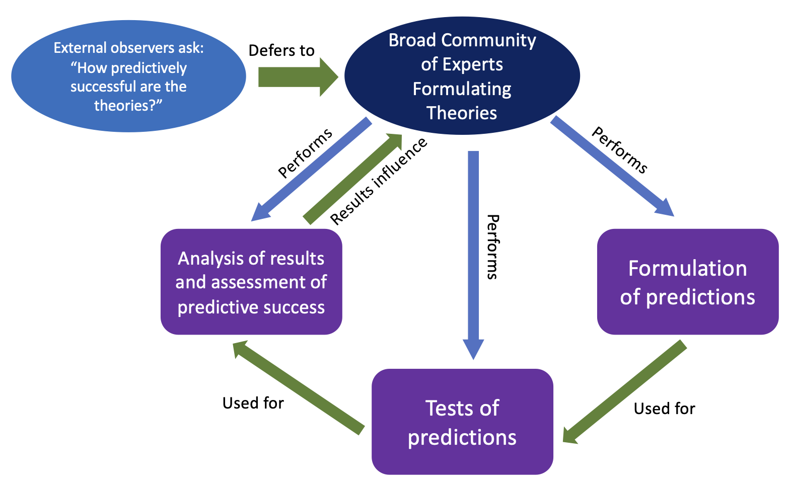
Our new contribution with this paper is to explore how one might build systems of incentives that optimally combine the advantages of group wisdom with the bias-mitigating influence of objective prediction assessments in prediction competitions. We hope that this fosters greater interest generally in the modeling of systems of experts operating within “adversarial collaboration” modes of interaction.
The Reward Algorithm
The setup of the reward system discussed in Rogers (2022) is that there is a sequence of questions with “yes” or “no” outcomes. Experts compete to provide the most accurately calibrated probabilistic prediction on each question. A reward \(r_{i,j}\) is given to each expert \(i\) for their performance on question \(j\). To motivate the discussion of the details below and organize the discussion, it is useful to begin with the following schematic formula,
| \[ r_{i,j} \propto (Prediction \; Accuracy) \times (Question \; Significance) \times (Consensus \; on \;Result)\] | \[(1)\] |
Prediction accuracy
We begin with the first factor in Equation 1. In this paper, we use the word “prediction” in the strict sense of section 2 from (Edmonds et al. 2019). Namely, a prediction is a statement about the probability of finding a result, usually based on a deeper set of theoretical ideas, that is made before the result is known. For example, a community of medical scientists might be testing whether a certain drug will return a null result in a specific trial. Then, an individual scientist might predict with, say, \(90\)% confidence, based on their understanding of the underlying biochemistry, that a non-null result will be found.
Each expert in the prediction competition is to be rewarded for providing the most accurate (or most calibrated) prediction possible for each question. By this we mean that the probability provided for a “yes” outcome should come as close as possible to the true probability, given all available knowledge. With all other factors in Equation 1 fixed, we might choose the reward to be proportional to a proper forecasting rule. For the algorithm in this paper, we use surprisal for “\(\text{Prediction Accuracy}\),” defined as
| \[ s_{i,j} = \begin{cases} -\ln p_{i,j} \, & \text{if outcome} \; = \text{yes} \\ -\ln (1-p_{i,j}) \, & \text{if outcome} \; = \text{no} \\ \end{cases} \, ,\] | \[(2)\] |
A limitation of Equation 2 with respect to a self-governing algorithm is that the experts in real-life debates frequently disagree about what the outcomes of predictions actually are (see the discussion in the introduction). In the absence of external referees, it is necessary to have some proxy for the yes or no “outcome” on the right side of Equation 2. We will defer to the expert wisdom of the crowd for this and define what we call the “resolution” \(v_{i,j}\) of expert \(i\) on question \(j\) as:
- \(v_{i,j} = +1\) if expert \(i\) believes or asserts that the outcome was “yes”
- \(v_{i,j} = -1\) if expert \(i\) believes or asserts that the outcome was “no”
- \(v_{i,j} = 0\) if expert \(i\) supplies no answer.
The mean of all experts’ resolutions regarding question \(j\) is then:
| \[ V_j = \frac{1}{N_j} \sum_i^{N_j} v_{i,j}\] | \[(3)\] |
| \[ q_j = \begin{cases} \text{yes (+1)} \,& \text{if} \;\; V_j > 0 \\ \text{no (-1)} \, & \text{if} \;\; V_j < 0 \\ 0 \, & \text{if} \;\; V_j = 0 \, \end{cases}\] | \[(4)\] |
Now we may write a less ambiguous version of Equation 2, appropriate for our purposes,
| \[ s_{i,j} = \begin{cases} -\ln p_{i,j} \, & \text{if} \;\; q_j = +1 \\ -\ln (1-p_{i,j}) \, & \text{if} \;\; q_j = -1 \\ 0 \, & \text{if} \;\; q_j = 0 \, \end{cases}\] | \[(5)\] |
Of course, the reliability of this measure of predictive success now depends on the reliability of the group consensus. Later, we will find that the numerical value of \(s_{i,j}\) in the \(q_j = 0\) case has no effect on the reward, but we fix it to zero in Equation 5 to have a definite algorithm.
Since some question outcomes in real-life scenarios will be much more difficult to predict than others, the reward given to an expert for their accuracy should depend on their surprisal relative to that of their peers, rather than on their absolute surprisal. To quantify this, we calculate the mean, the mean-squared, and the standard deviation of all surprisals for all experts on question \(j\),
| \[\begin{aligned} \langle s_j \rangle &= \frac{1}{N_j} \sum_i^{N_j} s_{i,j} \\ \langle s_j^2 \rangle &= \frac{1}{N_j} \sum_i^{N_j} s_{i,j}^2 \, \\ \Delta s_j &= \sqrt{\langle s_j^2 \rangle-\langle s_j \rangle^2} \end{aligned}\] |
\[(6)\] \[(7)\] \[(8)\] |
An expert’s reward should be large if their surprisal is far below what can be considered a large surprisal on question \(j\). The exact size of suprisal that we consider “large” here is somewhat arbitrary, but typically it will be some number \(c\) of standard deviations above the mean surprisal \(\langle s_j \rangle\) of the group on question \(j\). Therefore, we define a big surprise on question \(j\) to be
| \[ s^{\text{Big}}_j = \langle s_j \rangle + c \Delta s_j\] | \[(9)\] |
To summarize, we will make the reward for player \(i\) on question \(j\) proportional to the distance of their surprisal below the big surprisal \(s^{\text{Big}}_j\),
| \[ r_{i,j} \propto s^{\text{Big}}_j - s_{i,j}\] | \[(10)\] |
Question significance
The purpose of the reward algorithm is to incentivize adversarial collaboration in the prediction making process. However, if all experts are equally surprised by an outcome, that is if \(\Delta s_{j} \approx 0\) on question \(j\), then the critical adversarial component is missing. The reward system should incentivize question-prediction sequences that tend to demonstrate one set of ideas’ predictive advantages over anothers’. Thus, to account for the second factor in Equation 1 we also make the reward for expert \(i\) on question \(j\) proportional to the overall \(\Delta s_j\) for that question,
| \[ r_{i,j} \propto \Delta s_j\] | \[(11)\] |
An expert can expect to obtain a large reward only if \(\Delta s_j\) is reasonably large. The group of experts cannot use trivial or irrelevant predictions to inflate their overall reward count.
Consensus regarding results
It is frequently the case that real life experts do not agree on whether a particular prediction was confirmed or refuted by observations or measurements (O’Hagan 2019). Sometimes this might be because the original questions were vaguely formed. In other cases, there is disagreement over the details of how measurements were made or how data should be interpreted. This limits the reliability of the surprisal by itself, as it is calculated in Equation 5, as a measure of predictive accuracy. Robust collaborative efforts are necessary to avoid such scenarios and ensure that a reasonably broad consensus is established for each question and prediction cycle. Therefore, the amount of reward distributed should be weighted less if there is only weak consensus.
The absolute value of the mean resolution in Equation 3 is a quantitative measure of the consensus. If all experts agree that the outcome of prediction \(j\) was “yes,” then \(V_j = +1\), while if all agree that it was “no,” then \(V_j = -1\). If half of experts believe the outcome was “yes” and the other half believe it was “no,” then \(V_j = 0\), and there was no consensus. Thus, to account for the last factor in Equation 1, we will make the reward proportional to \(|V_j|\):
| \[ r_{i,j} \propto | V_j |\] | \[(12)\] |
We will refer to \(| V_j |\) as the “consensus” for question \(j\). A consensus of 1 means that all experts agree the result was either “yes” or “no.” A consensus of 0 means the experts are exactly evenly split. In the latter case, there is no way to determine a surprisal, and no reward points are given out.
Summary: The reward formula
To summarize the above, the reward for expert \(i\) on question \(j\) is to be simultaneously proportional to \(s_j^\text{Big} - s_{i,j}\) (Equation 10), \(\Delta s_j\) (Equation 11), and \(|V_j|\) (Equation 12). Substituting these into Equation 1 gives our final version of the reward formula:
| \[ r_{i,j} = \left(s_j^\text{Big} - s_{i,j}\right) \Delta s_j |V_j|\] | \[(13)\] |
In order for any individual expert to accumulate a large reward, the group must regularly reach consensus through collaboration. Otherwise, \(|V_j|\) will tend to be small. There must also be an adversarial element to each question-prediction cycle. Otherwise, \(\Delta s_j\) will be small and again the ability for any expert to accumulate a significant reward will be limited. Finally, each expert must supply an earnest and carefully considered prediction for each question or risk having a trend of small \(s_j^\text{Big} - s_{i,j}\). Thus, Equation 13 rewards the full constellation of behaviors we set out to incentivize with Equation 1.
Summing Equation 13 over all players gives the total amount of reward distributed for question \(j\),
| \[ r_{\text{total},j} = \sum_{i = 1}^{N_j} r_{i,j} = c N_j \Delta s_j^2 |V_j|\] | \[(14)\] |
Here, \(N_j\) is the total number of experts involved in answering question \(j\). To arrive at Equation 14, note from Equation 6 that:
| \[ \sum_{i=1}^{N_j} s_{i,j} = N_j \langle s_j \rangle\] | \[(15)\] |
Applied to Equation 13, this gives
| \[ \sum_{i = 1}^{N_j} r_{i,j} = N_j \left(s_j^\text{Big} - \langle s_{j} \rangle\right) \Delta s_j |V_j|\] | \[(16)\] |
But, from Equation 9, \(s_j^{\text{Big}} = \langle s_j \rangle + c \Delta s_j\), which substituted into the parentheses in Equation 14 gives Equation 14. Equation 14 establishes an interpretation for \(c\). It fixes the average reward per expert on question \(j\). If \(c\) is very large and positive, then all experts will tend to receive at least some positive reward, even for relatively inaccurate predictions. If \(c = 0\), then the total reward handed out is zero, and it becomes a zero sum prediction competition. In that situation, every reward point earned by one expert is accompanied by a negative reward (a reward penalty) for another. We will fix \(c = 1\) for now. This ensures that only a consistent pattern of extremely poor predictions can lead to a net negative reward for an expert. It is perhaps interesting that the total reward in Equation 14 is quadratic in the spread \(\Delta s_j\) in surprisal. This is because it enters in two places in the reward algorithm: i) in the measure of risk take by each expert relative to the group through the factor of \(\Delta s_j\) and ii) in the determination of what constitutes a large surprisal for the group as a whole through the factor of \(\left(s_j^\text{Big} - s_{i,j}\right)\).
After \(n\) predictions, the total reward accumulated by expert \(i\) will be represented with a boldface \(\mathbf{r}_i\),
| \[\mathbf{r}_i \equiv \sum_{j=1}^n r_{i,j}\] | \[(17)\] |
Of course, each expert will try to maximize their own \(\mathbf{r}_i\).
To understand the incentive structure this algorithm is designed to create, notice that for any given question it is not known to any of the experts what the total reward available to be distributed will ultimately be. To maximize the chances that both Equations 13 and 14 will be large, the experts are incentivized to collaborate to ensure that the following conditions hold:
- They must seek out questions where there is widespread disagreement within the group about what the outcome of the question might be, thus ensuring that the \(\Delta s_j^2\) in Equation 14 will be large. This is the “adversarial” component of “adversarial collaboration.”
- The group must be able to work together effectively to determine how to agree upon an outcome to the question after the relevant test or study is performed, thus ensuring that the consensus \(|V_j|\) on question \(j\) is likely to be close to one. This is the “collaboration” component of “adversarial collaboration.”
- The question must be interesting or relevant enough to attract many participants, thus maximizing \(N_j\).
It is assumed that the total reward distributed on each question is announced to all experts after that question is completed, thus guiding experts’ actions in predicting future questions.
A Basic Demonstration
Let \(\rm T\) stand for a specific theoretical belief or hypothesis that can either be true or false (\(\rm T\) stands for “theory”). For the purposes of illustration, we will assume that \(\rm T\) is objectively true and that belief in it therefore increases an expert’s ability to predict the outcomes of general predictable questions.
Belief and prediction accuracy
The basic setup of the simulation is that there are \(N\) experts competing on each question, and there are \(n\) total questions with “yes” or “no” outcomes. In our simulations, we will generate the outcomes \(\omega_j\) for the questions randomly, with \(\omega_j = 1\) corresponding to “yes” and \(\omega_j = -1\) corresponding to “no”.
Each player \(i\) has a list of attributes, the most basic of which is their level of belief in \(\rm T\). If they have a strong belief in \(\rm T\), then their probabilistic forecasts \(p_{i,j}\) for \(\omega_j\) will tend, on average, to be close to 1 when \(\omega_j = +1\) and close to zero when \(\omega_j = -1\). If they actively disbelieve \(\rm T\), then the situation is reversed; their forecasts will tend to be close to 0 when \(\omega_j = +1\) and close to 1 when \(\omega_j = -1\). For simplicity, we will quantify degree of belief \(d_i\) discretely with
| \[ d_i = \begin{cases} +4 \, & \text{strongest belief} \\ +3 \, & \text{strong belief} \\ +2 \, & \text{moderate belief} \\ +1 \, & \text{weak belief} \\ 0 \, & \text{undecided} \\ -1 \, & \text{weak disbelief} \\ -2 \, & \text{moderate disbelief} \\ -3 \, & \text{strong disbelief} \\ -4 \, & \text{strongest disbelief} \\ \end{cases}\] | \[(18)\] |
To generate a forecast for expert \(i\) on question \(j\), we will first generate a random real number \(\nu\) in the range \(\left( 0,1\right)\). Then,
| \[ p_{i,j} = \begin{cases} p(\nu,d_i) & \text{if} \;\; \omega_j = +1 \, (\text{true}) \\ 1 - p(\nu,d_i) & \text{if} \;\; \omega_j = -1 \, (\text{false}) \end{cases}\] | \[(19)\] |
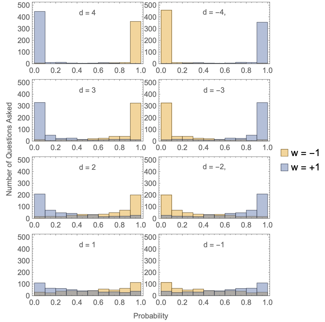
| \[ p(\nu,d_i) = \begin{cases} 1 - \nu^{21} & d_i = 4 \, \\ 1 - \nu^{5.3} & d_i = 3 \, \\ 1 - \nu^{2.7} & d_i = 2 \, \\ 1 - \nu^{1.6} & d_i = 1 \, \\ 1 - \nu & d_i = 0 \, \\ \nu^{1.6} & d_i = -1 \, \\ \nu^{2.7} & d_i = -2 \, \\ \nu^{5.3} & d_i = -3 \, \\ \nu^{21} & d_i = -4 \, \\ \end{cases}\] | \[(20)\] |
The power of \(\nu\) for each degree of belief in Equation 20 is chosen so that the average probabilities associated with each \(d_i\) are separated by even increments of approximately \(11.4\%\). An undecided expert (\(d=0\)) will assert an average probability of \(p(\nu,d=0)=50\%\), \(d = 1\) will have an average \(p(\nu,d=1)=61.4\%\), and so on up to approximately \(95\%\) for \(d = 4\). Degrees of disbelief (\(d < 0\)) are the mirror image of the degrees of positive belief, so that the average \(p(\nu,-d)\) is the average \(1-p(\nu,d)\). The questions that make up the prediction competition are intended to have at least some degree of uncertainty, so we will prohibit experts from asserting probabilities above or below some threshold. In our simulations of the next section, this threshold will be \(1.0\%\), so that \(p_{ij}\in [0.01,0.99]\).
Ideally, the degree of belief that we have labeled \(d_i\) would take on a continuous range of values rather than the discrete increment scheme we have used here. We may approximate the continuum limit of belief by using a larger number of increments. However, the computational time necessary grows rapidly for increments of more than about 9. When the number of increments is less than about 7, we find increasingly wild variation in results from one simulation to the next. Our choice above of 9 increments is a compromise between approximating the degree of belief as a continuum and maintaining a manageable computational time for our simulations. Note that we need an odd number of increments in order to have a totally uncertain belief level (\(d_j = 0\)) while having symmetry between belief and disbelief.
Histograms illustrating typical forecasts are shown Figure 2 for different degrees of belief. Note that they are symmetric under a change in \(\rm T\) from true to false. In the types of scenarios we are considering, each question might involve a complicated mixture of different beliefs regarding other relevant factors aside from \(\rm T\). A significant belief in \(\rm T\) pushes an expert toward highly calibrated predictions on average, but it does not guarantee an accurate prediction for each question. This means experts will be somewhat hesitant to update their beliefs, even after receiving low rewards, particularly if they are each aware of the presence of bias throughout the group.
Updating beliefs
After each question-prediction-outcome cycle, there is some chance that each expert will update their belief in \(\rm T\). To mimic typical human expert behavior, we will simulate the process of updating by separating it into the following two steps.
Random walk updating
The baseline scenario is that experts are highly unlikely to update their beliefs. In the absence of any external motivating factor, an expert will only increase or decrease their degree of belief randomly and with a small probability. We will call this probability the “mutation rate” and we will label it by \(\mu\). The value of \(\mu\) is fixed to be between \(0\) and \(1\). Then, the simulation first generates a random number \(\nu\) and if \(\nu < \mu\) it assigns \(d_{i,j+1} = d_{i,j} + 1\) (unless \(d = 4\)). It then generates another random number \(\nu\) and if \(\nu < \mu\) it assigns \(d_{i,j+1} = d_{i,j} - 1\) (unless \(d = -4\)). Therefore, if there were no other updating, each expert’s belief would be a random walk. In most of our simulations, we will use \(\mu = 0.01\). Thus, after each prediction an expert has a \(2\%\) chance of shifting their belief up or down one unit. Given a small mutation rate, and no other factors, the beliefs of the experts will slowly drift away from an initial consensus until they are totally randomized.
Reward motivated updating
In our simulations, our aim is to observe what happens when we tie belief updates to the reward formula in Equation 13. The basic assumption behind the simulation is that an expert with a low reward will tend to realign their belief to more closely match that of the experts with higher rewards. To express this in symbols, let \(i = M_j\) correspond to the expert with the highest (maximum) total accumulated reward at question \(j\). Then, \(\mathbf{r}_{M_j,j}\) is the maximum reward held by any expert by question \(j\), and \(d_{M_j,j}\) is the degree of belief held by the expert with the maximum reward. Other experts will update their beliefs if their reward falls some distance below what might be considered a “large” reward. Depending on the personality traits of the specific expert, a large reward might mean anything above the mean reward, or it could be something close to \(\mathbf{r}_{M_j,j}\). We will compromise between these two ways that experts might compare themselves to their peers and define a “large” reward to be the weighted average of \(\mathbf{r}_{M_j,j}\) and \(\langle \mathbf{r}_j \rangle\),
| \[ \mathbf{r}_j^\text{Large} = x \langle \mathbf{r}_j \rangle + y \mathbf{r}_{M_j,j}\] | \[(21)\] |
An individual expert’s “reward deficit” \(\delta \mathbf{r}_{i,j}\) will be how far below \(\mathbf{r}_j^\text{Large}\) their accumulated reward at question \(j\) falls,
| \[\delta \mathbf{r}_{i,j} = \mathbf{r}_j^\text{Large} - \mathbf{r}_{i,j}\] | \[(22)\] |
Each expert will have a high probability of updating their belief if their reward deficit is a critical fraction of \(\mathbf{r}_j^\text{Large}\). The farther their reward falls below the large reward, the less likely they are to retain their prior belief. We implement this with the formula,
| \[\begin{aligned} d_{i,j+1} = \begin{cases} d_{i,j} & \nu \leq e^{-a_j \frac{\delta \mathbf{r}_{i,j}}{\mathbf{r}_j^\text{Large}}} \\ d_{i,j} + \text{sign}(d_{M_j,j}- d_{i,j}) & \;\text{otherwise} \end{cases}\end{aligned}\] | \[(23)\] |
Since experts are only likely to update beliefs in situations where reasonably large rewards are available, we will not choose a fixed number for \(a_j\), but instead write:
| \[ a_j = a_0 \frac{r_{\text{total},j}}{r_{\text{total},j} + r_0}\] | \[(24)\] |
The value of \(r_0\) is a threshold reward that we will fix later. If the total award distributed on question \(j\) is large relative to \(r_0\), then the affinity is \(a_j \approx a_0\). If the total reward is close to zero, then \(a_j \approx 0\).
Modeling consensus and bias
If the objective outcome \(\omega_j\) of a prediction turns out not to match an expert’s expectations, they may be inclined to reject the objective outcome and instead choose a \(v_{i,j}\) that is more in line with their prior beliefs. This bias effect also needs to be modeled in our simulations. To do so, we assume that if expert \(i\)’s surprisal is much larger than the mean on question \(j\), then they will reject the objective outcome and choose instead \(v_j = - \omega_j\).
To express this in a formula, define a surprisal \(\hat{s}_{i,j}\) that is calculated exactly as in Equation 5, but now using \(\omega_j\) rather than \(q_j\) (We can call this the “objective surprisal” since it is based on the objective underlying reality rather than the expert consensus). Then, we determine the validation number of expert \(i\) on question \(j\) by using:
| \[ v_{i,j} = \begin{cases} \omega_j & \text{if}\;\; \nu \leq e^{ -b \left( \frac{\hat{s}_{i,j}}{\langle \hat{s}_j \rangle + b_0}\right)} \\ -\omega_j & \text{otherwise} \end{cases}\] | \[(25)\] |
If, on one hand, the average objective surprisal is large, \(\langle \hat{s}_j \rangle \gg b_0\), then all or most of the experts have made an inaccurate prediction, and so they likely hold the wrong belief. In this case, it is only \(b\) that matters in Equation 25. In this case there is a probability of \(\approx e^{-b}\) that an expert with a typical objective surprisal will agree with the objective outcome. Thus, \(b\) represents a collective, group bias.
On the other hand, if the group of experts is mostly correct in their predictions, so that \(\langle \hat{s}_j \rangle \ll b_0\), then \(\langle \hat{s}_j \rangle\) becomes irrelevant in Equation 25. Only the handful of experts with poor predictions will be likely to reject the objective outcome, and their probability for accepting the objective outcome is \(\approx e^{-b/b_0}\). Thus, \(b/b_0\) is a measure of individual biases against a correct group consensus.
For moderate \(\langle \hat{s}_j \rangle\), Equation 25 interpolates between the two scenarios above.
We will simply call the parameter \(b\) the “bias” of the experts. Since we are mainly interested in the effect of collective bias for now rather than individual biases, we will set:
| \[ b_0 = 0.7\] | \[(26)\] |
A surprisal of \(s \approx 0.7\) is the result of a \(p \approx 0.5\) forecast. We will study the effect of changing \(b_0\) below. If \(b\) is large, then expert \(i\) will only match their \(v_{i,j}\) to \(\omega_j\) when their objective surprisal is small relative to \(\hat{s}_{i,j} \ll \langle \hat{s}_j \rangle + b_0\). If \(b \approx 0\), then the experts will almost always agree with the correct, objective outcome. If \(b \approx \infty\), the experts will always disagree with the objective outcome whenever \(\hat{s}_j > \langle \hat{s}_j \rangle\).
Exit criterion
In real-world scenarios, groups of experts will usually cease to question an underlying theory \(\rm T\) once beliefs have stabilized and the potential for large rewards has vanished. To simulate this, we will halt the questions once:
| \[ r_{\text{total},j} < r_{j,\text{threshold}}\] | \[(27)\] |
In cases where stability is not reached, we exit the simulation after \(n_\text{max}\) questions. For this, we will omit “failed” questions, i.e., those for which the total rewards are exactly zero when \(V_j=0\). Later, we will estimate the value of \(r_{j,\text{threshold}}\) based on the behavior of 20 experts in a prediction competition.
Parameter selection
In our sample simulations, we choose parameters to represent reasonable expectations for the behavior of an actual group of experts competing to make accurate predictions. For statistical measures like average reward or average belief to be meaningful, the number of experts should be large but still realistic for an actual community of experts in a highly specialized subject. It also must be kept small enough for simulation times to be manageable. We will take \(N_j = 20\). If a typical small expert research group publishes articles with around 5 authors, then this would corresponds to a competition between about 4 research groups. If enough rewards points are distributed so that there is at least an approximately \(10\%\) probability per expert that a belief will be modified, then there is roughly an \(88\%\) chance that with each question a belief will be updated. If there is only a random walk, with a \(0.2\%\) chance for each expert to update on each question, then there is roughly a \(33\%\) chance that at least one expert’s belief will be updated on each question. Thus, over the course of several questions, we expect the distinction between \(2\%\) per expert (random walk) and \(\approx 10\%\) per expert to become evident. If there were a \(\lesssim 1/3\) chance of an \(r_{\text{total},j} < r_{j,\text{threshold}}\) entirely by random chance, then there is a \(\lesssim 0.01\%\) of having \(r_{\text{total},j} < r_{j,\text{threshold}}\) on three questions consecutively. Having \(n_\text{stable} \approx 4\) questions in a row where there is a very small reward is, therefore, a reliable indication that the group experts have converged upon a upon a stable degree of belief.
We also estimate that \(a_0 \approx 0.1-0.2\) is a reasonable affinity for describing a typical expert. To see why, consider an expert with \(\delta \mathbf{r}_{i,j} \approx \mathbf{r}_j^\text{Large}\) on question \(j\), and assume that \(r_{\text{total},j} \gg r_0\). Then from Equation 23 the probability that the expert shifts their belief \(d\) by one increment is approximately \(10\%-40\%\). Repeated over the course of five questions, this scenario yields a probability between \(41\%\) and \(97\%\) for the expert to increment their belief \(d\).
For the affinity related quantities in Equation 21, we make the choices:
| \[\begin{aligned} x={}&y=\frac{1}{2},\qquad r_0=50\end{aligned}\] | \[(28)\] |
We have estimated the value of \(r_0\) by considering the situation where, out of 20 experts, half of them have the strongest believe in theory \(\rm T\) (\(d=4\)), and the other half have the strongest disbelief (\(d=-4\)). Keeping fixed the degree of belief, we simulate an experiment with a large number of questions and calculate the total rewards \(r_{\text{total},j}\) at every step. The average over all questions is \(\langle r_{\text{total}}\rangle\approx 100\), which is an estimate for very large rewards given in a single question. Since this estimate applies to a rather extreme scenario, we take half of this value, \(r_0=\langle r_{\text{total}}\rangle/2\). We will estimate the effect of adjust \(x\) and \(y\) in the robustness section below.
For the exit criterion, we set:
| \[\begin{aligned} r_{j,\text{threshold}} ={}&4.04,\,\, n_{\text{stable}}=4,\,\, n_{\text{max}}=1000\end{aligned}\] | \[(29)\] |
For estimating reasonable ranges for the bias parameter \(b\), let us recall that when an expert’s surprisal is typical, \(\hat{s}_{i,j} \approx \langle s_j \rangle + b_0\), the probability that they will agree with the objective outcome is \(\approx e^{-b}\). Thus, an expert with \(b \lesssim 0.7\) is relatively unbiased while one with \(b \gtrsim 0.7\) is somewhat biased.
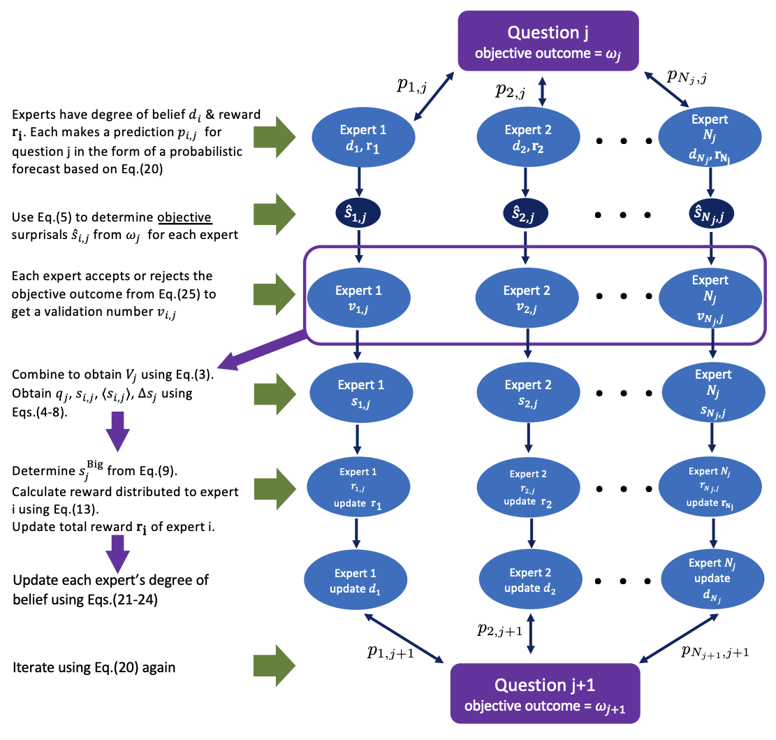
The steps described in this section are summarized in the pseudoalgorithm diagram shown in Figure 3.
Numerical Examples
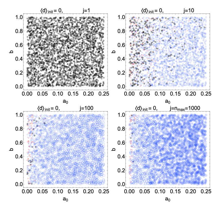
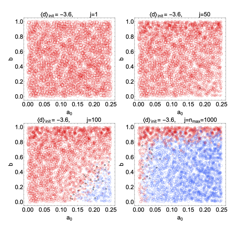
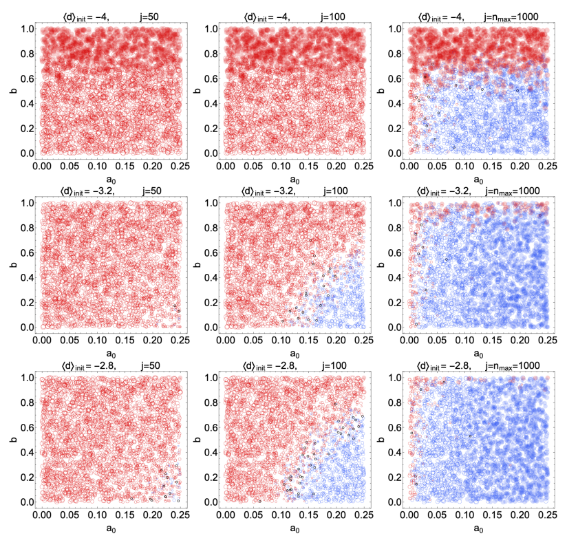
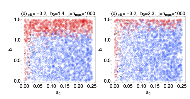
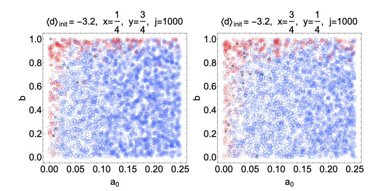
Figures 4 and 5 show the outcomes of simulations with 20 experts, with each panel corresponding to a different average initial \(d\). The vertical axes in each panel indicates the bias parameter \(b\) and the horizontal axes show the basic reward affinity parameter \(a_0\). Each red or blue circle represents the outcome of a single simulation, and its position in the graph is given by the values of \(b\) and \(a_0\) used in that simulation. A blue circle means that the final average \(d\) at the end of the simulation was positive (a correct belief in the truth of \(\rm T\)), while a red circle means the average belief is negative (disbelief in \(\rm T\)). A black circle means that the final average degree of belief was \(d=0\). If the stop condition was reached in a simulation, i.e., if the inequality in Equation 27 was satisfied for \(n_{\text{stable}}=4\) consecutive questions, we indicate this with a solid, filled circle. A large blue circle indicates a strong average final belief (\(d\) close to 4) while a small blue circle indicates weak average belief (\(d\) closer to 0). An analogous interpretation applies to the size of the red circles, with red indicating degrees of disbelief. The different panels in each figure show snapshots at intermediate steps of the simulations. For instance, Figure 4 shows the state of belief at questions \(j=1,10,100\) and \(j=n_{\text{max}}=1000\).
Figure 4 shows the outcomes of \(3000\) numerical simulations in a scenario where half of the \(20\) experts start with \(d = -4\) (strong disbelief) and half start with \(d = +4\) (strong belief). We use this to establish a baseline, since at a minimum the reward distribution algorithm should cause the group of experts to migrate toward the correct answer if they begin with evenly split beliefs in the correctness of \(\rm T\). Figure 4 confirms this basic trend. With a large affinity \(a_0 \gtrsim 0.15\) and a small bias \(b \lesssim 0.45\), the group quickly migrates toward belief in \(\rm T\) after only a handful of questions. After \(j=1000\) questions, the group always settles on belief in \(\rm T\), even when there is a large bias.
Figure 5 is a more interesting case. There, all but one of the 20 experts begin with a strong disbelief (\(d = -4\)) in \(\rm T\). A single contrarian expert has a \(d = +4\) belief. Naturally, many predictions are required to shift the belief of the majority into the \(d > 0\) region, but if \(a_0 \gtrsim 0.15\) and \(b \lesssim 0.4\), a shift is essentially guaranteed to begin at least around the \(100\) question mark. Even after 50 questions, the sizes of the red circles have begun to shrink in the lower right-hand corner of the plot, indicating that belief in \(\rm T\) has started to become more evenly split. As the number of predictions approaches infinity, the group is guaranteed to converge on belief in \(\rm T\) so long is \(a_0\) and \(b\) lie within the largely blue rectangular region of the \(j = 1000\) plot. Notice that, if \(b \gtrsim 0.85\), the group is unlikely to ever abandon its disbelief in \(\rm T\) regardless of how many predictions are made or how many questions are asked.
Here it is worth recalling what \(a_0\) and \(b\) quantify at the level of individual experts. The reward affinity \(a_0\) quantifies the experts’ willingness to update their level of belief in \(\rm T\) based on their predictive accuracy relative to their peers if they assume that the reward is an accurate measure of predictive power. Since that last assumption is nontrivial, and since it depends on the ability for the group to reach consensus and agree on the outcomes of predictions, then the value of \(a_0\) also quantifies the experts’ overall trust in the reward system. The value of \(b\) quantifies the experts’ tendency to disagree about the objective outcomes of each question/prediction cycle. Figure 5 shows that when the group has a large enough \(a_0\), the system can tolerate a relatively large bias \(b\) and still migrate toward the objectively correct conclusion (\(\rm T\) is true). Conversely, as long as \(b\) is very small, the group will migrate to the correct conclusion even with only a modest \(a_0\). The reliability only breaks down completely when there is a high bias (large \(b\)) and/or very little trust in the system (low \(a_0\)).
If all the experts begin with strong disbelief, then one should expect to require very many questions (and very low bias) before there is a shift in belief. Conversely, if more of the experts begin with \(d = 4\) (\(\rm T= \text{true}\)), then one should expect the transition from \(\langle d \rangle < 0\) to \(\langle d \rangle \geq 0\) to take place much faster. These trends are confirmed by Figure 6, where three additional scenarios are considered: \(i)\) all experts start at \(d=-4\) (top row), \(ii)\) 2 experts start at \(d=4\) and the rest at \(d=-4\) (central row), \(iii)\) 3 experts start at \(d=4\) and the rest at \(d=-4\) (bottom row). Scanning from top to bottom, the transition from disbelief to belief (at large \(a_0\) and small \(b\)) happens at earlier \(j\). If \(3/20\) of the experts begin with a strong belief in \(\rm T\) (bottom row) , and \(b \lesssim 0.25\), \(a_0 \gtrsim 0.2\), the transition begins already by \(j = 50\). Importantly, the top row confirms that the transition from disbelief to belief eventually occurs even if all the experts start with strong disbelief. All that is required is that \(b \lesssim 0.6\).
Robustness
Having just illustrated the basic operation of the reward algorithm, we briefly investigate the effects of modifying some of the assumptions used in the sample model of expert behavior above and confirm that these do not significantly alter the main qualitative trends observed above.
Finite and discretization effects
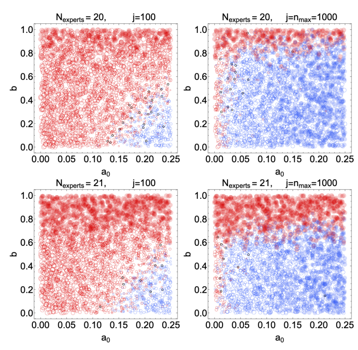
As a measure of predictive power, the reward algorithm is optimal in the limit of infinite experts and predictions. With finite numbers of experts and predictions, the input to Equation 13 is granular. Examining the impact of this granularity can help with solidifying othe understanding of the reward algorithm in Equation 13 For example, if all experts supply definite resolutions as in our model, then the unusual case of an exactly zero mean resolution (\(V_j=0\)) and consensus is only possible with an even number of experts, as in our simulations above. With an odd number of experts, there is guaranteed to be a definite result or \(q_j\) on each question. In Figure 8, we test the impact of having an odd number of experts by adding a single initial low-belief expert. Qualitatively, the behavior over many predictions reflects expectations, though the bias above which the group fails to converge on the correct belief is significantly lower, around \(0.6\) (for large \(a_0\)) rather than \(0.8\) for \(N_j=21\) compared to \(N_j=20\).
This difference is due to the fact that we have excluded “failed” questions (corresponding to \(|V_j|=0\)) in the exit criterion, which can only take place in cases with an even number of experts. For \(N_j =\) even, a significant number of questions may have \(|V_j|=0\) once the experts are nearly evenly split, but these questions never count towards the consecutive \(n_{\text{stable}}\) needed to reach stability and exit the simulation. By contrast, for \(N_j=\) odd, the smallest possible value for the mean resolution is \(|V_j|=1/N_j\), so no question is excluded. As a result, the effect of the initial bias is amplified – the chance to trigger the exit criterion early is larger for \(N_j\) odd, so the average degree of belief can remain negative at the end of a simulation more often. This is specially visible in Figure 8, by examining the region \(b\approx0.8\): For \(N_j=20\), at question \(j=100\) (top-left panel), the large number of open red circles indicates that few points have reached stability, while for \(N_j=21\) (bottom-left panel), nearly all have reached stability. Still, while the nonbelief-to-belief transition occurs at a somewhat different \(b\), the general trend that we aim to exhibit is unaffected. Furthermore, we have checked that runs with \(N_j = 19\) are nearly indistinguishable from those with \(N_j = 21\), and likewise runs with \(N_j = 20\) are nearly indistinguishable from those with \(N_j = 22\).
The probability for exactly \(|V_j| = 0\) decreases as the number of experts grows, though it always remains significant at a cusp where experts are nearly evenly split in their beliefs. To keep these proof-of-principles simulations simple, we have not yet allowed experts to register null resolutions – the \(v_{i,j} = 0\) option discussed above Equation 3 is thus far excluded in Equation 25. In future extensions of our work, we plan to incorporate this possibility, in which case we expect the difference between even and odd \(N_j\) to vanish. Furthermore, having a failed question correspond to \(|V_j| = 0\) exactly may be overly restrictive. An improvement might be to instead require \(|V_j|\) to be larger than some threshold \(V_{\min}\). We plan to further investigate the impact of “null” resolutions in future iterations of this work.
Mutation rate
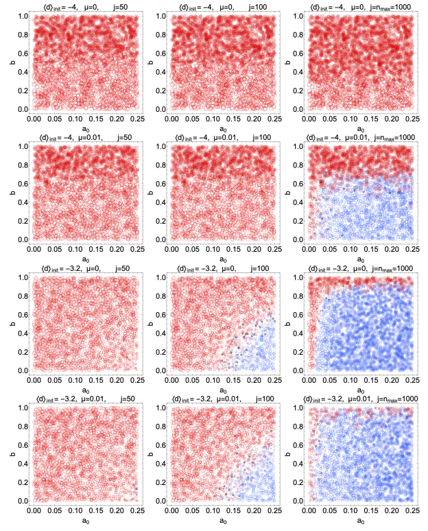
An important parameter is the mutation rate, \(\mu\), which was fixed at \(0.01\) in all simulations above. The purpose of the mutation rate was to model the rather random ways that individual experts will naturally modify their views independently of external pressure or direct evidence. If the mutation rate is set exactly to zero, experts will only update their beliefs by comparing their own cumulative reward counts with those of other experts. Thus, once all experts have obtained the same degree of belief \(d\), there can be no more updating. A nonzero mutation rate is necessary if the group of experts is to break away from an initially absolute consensus. Increasing \(\mu\) causes beliefs to migrate more rapidly, but the cost is that random variations in belief persist even as the number of predictions increases. We illustrate these trends in Figure 7. Each column shows simulations at \(j = 50\), \(100\) and \(1000\) predictions respectively. On the first row, all experts start with extreme disbelief in \(\rm T\) (\(d = -4\)), and the mutation rate \(\mu\) is fixed at \(0\). All circles remain red as the number of predictions increases, confirming that a mutation rate of \(0\) means the experts never migrate beyond the largest \(d\). The second row is the same as the first row, but now with a nonzero mutation rate \(\mu = 0.01\). For large \(a_0\) and small \(b\), the group migrates to belief in \(\rm T\), albeit only after many predictions. On the third line, we return to the case of \(\mu = 0\), but now we allow two of the experts to begin with strong belief (\(d = 4\)) in \(\rm T\), so that \(\langle d\rangle = -3.2\) at the outset. Now the two believing experts moving the group very decisively to the \(d > 0\) state unless \(b\) is very large (\(b \gtrsim 1.0\)) or \(a_0\) is very small (\(a_0 \lesssim 0.01\)). Since there are no random fluctuations in \(d\) here, the transition between the blue and red regions is sharply defined, and the circles tend to be solid. Finally, on the last row we repeat the simulation of the third row but with \(\mu = 0.01\). The group moves toward the \(d > 0\) region again here. Indeed, there is only a small difference from the third row. Primarily, it is that the line separating the blue and red regions is slightly less clearly defined, given the increase in random fluctuations.
To summarize, a small but nonzero \(\mu\) is sufficient to guarantee that the group will migrate toward \(d > 0\), even if all experts start with \(d = -4\). A decisive final consensus is likely so long as \(\mu\) is no larger than a few percent.
Threshold bias
Experts will almost always correctly validate the outcome of a prediction if they have \(\hat{s}_{i,j} \ll b_0\). However, for much larger surprisals they will be strongly influenced by their biases. We originally chose \(b_0 = 0.7\) because this corresponds to the surprisal in a prediction with approximately 50\(\%\) odds, so any surprisal larger than roughly \(0.7\) may reasonably be considered “surprising” for a typical expert in the absence of any other considerations. However, actual experts may (and will likely) operate with different effective surprisal thresholds. A level of surprise that is acceptable to one expert may be intolerable to another. The assumption that any suprisal above \(0.7\) may be considered large is rather conservative. A more realistic scenario is that most experts can accept surprisals somewhat larger than \(0.7\).
A probability threshold of \(p \gtrsim 75\%\) corresponds to \(b_0 \approx 1.4\) and a probability threshold of \(p \gtrsim 90\%\) corresponds to \(b_0 \approx 2.3\). We expect the blue portion of the \(b\) versus \(a_0\) plots to increase in size if we use these larger values of \(b_0\). We confirm this by repeating the simulations corresponding to the scenario where all experts start with \(d = -4\), with each of these new surprisal thresholds, and we show the results in Figure 9.
What constitutes a “large” reward?
To calculate the likelihood that experts modify their beliefs, we needed to establish a standard against which they may compare their reward counts with those of other experts (recall the discussion around Equation 21). The possibilities were: i) experts compare their total reward counts with that of the group as a whole or ii) experts compare their total reward counts with that of the “winner,” i.e., the member of the group with the largest reward. Both options reflect influences that likely affect actual experts, and in real world groups it is likely a combination of the two, with the prevalence of each depending on the details of the specific group of experts. In our simulations, we compromised by taking a linear combination of i) and ii) and weighting each equally (see Equation 21). Our last robustness test will be to examine the sensitivity to this choice of the proportion of i) and ii). In Figure 10, we show the effect using the combinations \((x,y) = (3/4,1/4)\) and \((x,y) = (1/4,3/4)\) in Equation 21 rather than the \((x,y) = (1/2,1/2)\) that we used earlier. We have repeated the scenario in the last row of Figure 7, apart from the change in \((x,y)\). Namely, we start with \(d = -4\) for all experts except two, who start with \(d = 4\).
Figure 10 shows that, perhaps surprisingly, there is very little effect on the qualitative behavior of the \(b\) versus \(a_0\) phase diagrams from modifying the exact values of \(x\) and \(y\)
Discussion and Future Directions
The simulations above effectively illustrate the main principles behind the reward algorithm proposed in Equation 13, and they show that it performs as designed under reasonable assumptions concerning the model of the expert group. If the group is collectively driven to gather large reward points (as expressed through a large \(a_0\)), and has a low bias (small \(b\)), then the group migrates toward the factually correct theory \(\rm T\). The important point for our purposes is that this is driven by the collective interaction between the participants and does not require an external referee to determine the true outcome or relevance of each prediction. It is in this sense that the reward algorithm is “self-governing”. To reproduce the simulations, the relevant Wolfram Mathematica documents may be found here: https://drive.google.com/file/d/1CE4WNy9XRZHF94WN3XkRW5kGkalddsLl/view.
Naturally, there is still a great deal of stress-testing that still needs to be performed. One way to do this is to add complexity to the model of the interaction between experts. For example, it may be instructive to consider more complex models than Equations 23-25, for the probability distributions that determine whether experts switch their beliefs or fail to reach a consensus. Furthermore, the group of experts might be made more realistic by assigning a bias and affinity to each individual expert rather than to the group of experts as a whole. One may then investigate the effect of increasing both the magnitude of the bias and the number of individuals with a large/small bias. One of the limitations of our simulations so far is the relatively small number of experts (\(20\)) involved in the simulated prediction competition. Further insight might be gained by increasing this number.
The simulations above fall primarily under the “illustration” category in the classification scheme of Edmonds et al. (2019). To go beyond basic proofs of principle will require entirely separate simulations with more sophisticated methods dedicated to specific purposes (Bonacich & Lu 2012; Miller & Page 2009). To explore and better understand the behavior of realistic scientific communities under the influence of various prediction incentives, accounting for heterogeneity certainly becomes important (Squazzoni et al. 2014), and agent-based models are likely the appropriate approach. As emphasized in Section 2, the novel element of the reward system of Section 3 that these future simulations will need to address is the feedback between a group’s success in making prediction and their ability to assess the outcomes of those predictions correctly.
Here, we also hope to find guidance in existing bodies of research into group consensus formation (Adams et al. 2021; Groeber et al. 2009; Hegselmann et al. 2002; Lorenz 2006; Mavrodiev et al. 2013; Weinans et al. 2024; Zhang et al. 2021) when modeling trends toward certain values of the measure we have called \(V_j\).
We intend to implement these extensions in future updates. Our long term hope is for this and future outgrowths of this work to become useful for guiding modifications, refinements or other updates to the algorithm in Equation 13. We also hope that our current work attracts outside interest, particularly from experts in social modelling and simulations, in this and in the broader problem of understanding and improving incentive structures in predictive sciences.
Acknowledgements
This work was supported by a Program for Undergraduate Research and Scholarship (PURS) grant from the Office of Research and Perry Honors College at Old Dominion University, Norfolk, Virginia, USA. We especially thank Yaohang Li, Lucia Tabacu, and Balsa Terzic for many useful discussions that helped guide this work. We also thank the referees from JASSS who have helped us to substantially improve the quality of our paper.References
ADAMS, J., White, G., & Araujo, R. (2021). The role of mistrust in the modelling of opinion adoption. Journal of Artificial Societies and Social Simulation, 24(4), 4. [doi:10.18564/jasss.4624]
ALDOUS, D. J. (2019). A prediction tournament paradox. The American Statistician, 00, 1–6.
BATEMAN, I., Kahneman, D., Munro, A., Starmer, C., & Sugden, R. (2005). Testing competing models of loss aversion: An adversarial collaboration. Journal of Public Economics, 89(8), 1561–1580. [doi:10.1016/j.jpubeco.2004.06.013]
BONACICH, P., & Lu, P. (2012). Introduction to Mathematical Sociology. Princeton: Princeton University Press.
BURGMAN, M. A. (2016). Trusting Judgements: How to Get the Best Out of Experts. Cambrige: Cambridge University Press. [doi:10.1017/cbo9781316282472]
CLARK, C. J., & Tetlock, P. E. (2021). Adversarial collaboration: The next science reform. In C. L. Frisby, R. E. Redding, W. T. O’Donohue, & S. O. Lilienfeld (Eds.), Ideological and Political Bias in Psychology: Nature, Scope, and Solutions. Berlin Heidelberg: Springer. [doi:10.1007/978-3-031-29148-7_32]
EDMONDS, B., Le Page, C., Bithell, M., Chattoe-Brown, E., Grimm, V., Meyer, R., Montañola-Sales, C., Ormerod, P., Root, H., & Squazzoni, F. (2019). Different modelling purposes. Journal of Artificial Societies and Social Simulation, 22(3), 6. [doi:10.18564/jasss.3993]
ELLEMERS, N., Fiske, S. T., Abele, A. E., Koch, A., & Yzerbyt, V. (2020). Adversarial alignment enables competing models to engage in cooperative theory building toward cumulative science. Proceedings of the National Academy of Sciences, 117(14), 7561–7567. [doi:10.1073/pnas.1906720117]
ELSENBROICH, C., & Polhill, J. G. (2023). Agent-based modelling as a method for prediction in complex social systems. International Journal of Social Research Methodology, 26(2), 133–142. [doi:10.1080/13645579.2023.2152007]
GNEITING, T., & Raftery, A. E. (2007). Strictly proper scoring rules, prediction, and estimation. Journal of the American Statistical Association, 102(477), 359–378. [doi:10.1198/016214506000001437]
GROEBER, P., Schweitzer, F., & Press, K. (2009). How groups can foster consensus: The case of local cultures. Journal of Artificial Societes and Social Simulations, 12(2), 4.
HEGSELMANN, R., Krause, U., & others. (2002). Opinion dynamics and bounded confidence models, analysis, and simulation. Journal of Artificial Societies and Social Simulation, 5(3), 2.
KYNN, M. (2008). The “heuristics and biases” bias in expert elicitation. Journal of the Royal Statistical Society Series A: Statistics in Society, 171(1), 239–264. [doi:10.1111/j.1467-985x.2007.00499.x]
LORENZ, J. (2006). Consensus strikes back in the Hegselmann-Krause model of continuous opinion dynamics under bounded confidence. Journal of Artificial Societies and Social Simulation, 9(1), 8.
MAVRODIEV, P., Tessone, C. J., & Schweitzer, F. (2013). Quantifying the effects of social influence. Scientific Reports, 3(1), 1360. [doi:10.1038/srep01360]
METACULUS. (2023). Metaculus. Available at: https://www.metaculus.com/questions/.
MILLER, J. H., & Page, S. E. (2009). Complex Adaptive Systems: An Introduction to Computational Models of Social Life. Princeton: Princeton University Press.
O’HAGAN, A. (2019). Expert knowledge elicitation: Subjective but scientific. The American Statistician, 73(1), 69–81. [doi:10.1080/00031305.2018.1518265]
PETROPOULOS, F., Apiletti, D., Assimakopoulos, V., Babai, M. Z., Barrow, D. K., Ben Taieb, S., Bergmeir, C., Bessa, R. J., Bijak, J., Boylan, J. E., & others. (2022). Forecasting: Theory and practice. International Journal of Forecasting, 38(3), 705–871.
RITCHIE, S. (2020). Science fictions: Exposing fraud, bias, negligence and hype in science. New York, NY: Random House.
ROGERS, T. C. (2022). A self-governing, self-regulating system for assessing scientific predictive power. arXiv preprint. Available at: https://arxiv.org/abs/2205.04503.
WEINANS, E., van Voorn, G., Steinmann, P., Perrone, E., & Marandi, A. (2024). An exploration of drivers of opinion dynamics. Journal of Artificial Societies and Social Simulation, 27(1), 5. [doi:10.18564/jasss.5212]
WITKOWSKI, J., Freeman, R., Vaughan, J. W., Pennock, D. M., & Krause, A. (2023). Incentive-compatible forecasting competitions. Management Science, 69(3), 1354–1374. [doi:10.1287/mnsc.2022.4410]
WOLFRAM RESEARCH (2022). Mathematica, Version 13.2. Available at: https://www.wolfram.com/mathematica.