The Role of Monetary Evaluation and Social Pressure Within the Residential Rooftop Photovoltaic Systems Diffusion Model PVact

Introduction

Motivation

With a share of 25.8% of the total final energy consumption in the EU in 2022 (Eurostat 2024), private households are an important factor in climate change mitigation. At the same time, the EU-wide economic potential for rooftop photovoltaic (PV) is estimated to be at least 680 TWh/year (Kakoulaki et al. 2024), of which residential buildings exhibit a significant share. Households thus play a crucial role both in final energy demand and generation and are central in reaching emission neutrality.

For this, a massive increase in rooftop PV capacity is needed and PV projects on every scale are required. In order to reach net-zero emissions, the IEA states the requirement to install an additional annual global capacity of 630 GW for PV alone (IEA 2021). While institutional decisions are shaped primarily by rational arguments and the public sector can be influenced by political will, private actors either need to be convinced or regulatory measures need to be taken. However, regulatory measures can be politically costly, as has been the case with the Gebäudeenergiegesetz¹ in Germany, showing the importance of political acceptance.

Human decision making is poorly described by rational choice theories (Vlaev 2018). Household adoption addresses decentralized decisions of rationally bounded actors whose decision depends on a range of interacting individual, social and cognitive factors.

Understanding consumer behavior and decision-making is crucial not only for successful product launch planning but also for effective policy design (Simões 2016). Paying attention to social acceptance and the policy making perspective can address challenges in acceptance of renewable energy technologies (Dermont et al. 2017). Understanding how innovations can be effectively launched and adopted is the focus of the field of innovation diffusion (see e.g. Rogers 2003), which can be supported by modeling approaches. For model-based strategic planning of product launches and policy instruments, different approaches exist. Of these, system thinking, system dynamics and agent-based modeling (ABM) appear to be the most appropriate for modeling complex dynamic systems and evaluating policies addressing these systems (Schuenemann, Johanning, Herold, et al. 2024). Detailed agent-based models of innovation diffusion have been shown to inform strategies directed at policy questions (Schuenemann, Johanning, Reger, et al. 2024). However, agent-based models often come with a number of shortcomings, such as failure to appropriately address empirical data, behavioural theories, spatiality and nuances of the physical environment and economic features (Alipour et al. 2021).

In order to address these shortcomings, the agent-based innovation diffusion framework IRPact (Integrated Resources Planning and interACTion) was developed (Johanning et al. 2020), aiming at easy and flexible development of models on the diffusion of sustainable products (see the section below). As an application to the diffusion of residential rooftop PV adoption, a granular municipal agent-based model PVact (PhotoVoltaic innovation diffusion and interACTion) was implemented, allowing for detailed investigation of the diffusion of residential rooftop PV systems by private households. The model is both empirically and theoretically grounded (in behavioral theories) and allows for high-grained spatiality, with \(\geq\) 48,000 agents corresponding to addresses in the respective GIS (geographic information system).

While modeling can be used to isolate the system components that the researchers believe to be essential to the dynamics and effects of interest, one has to be aware that a model is a simplification and reduction of the system under study. The goal of the PVact model is to identify the most important factors for PV adoption decision. However, as mentioned above, the literature shows that there is considerable uncertainty as to which factors are relevant for residential adoption of rooftop PV; decision factors that seem to be particularly important appear to be monetary evaluation, normative pressure, normative motives, opinion dynamics, advertisement, preferences, perceptions, values, beliefs, attitudes, norms, behavioral control, household demographics and social networks (see e.g., Vibrans et al. (2023), for a selection of major factors).

Contributing to more insight into the relative importance of these factors and the model dynamics associated with them would be a valuable contribution to the discourse.

While financial evaluation and normative pressure have been investigated with the use of PVact (Johanning et al. 2023), opinion dynamics, attitudes and the role of the social network have not yet been investigated within the framework. However, their interplay and their influence on system behavior are of considerable importance for understanding residential PV adoption.

Objectives and research interest

The adoption of rooftop PV in residential socio-techno-economical contexts has shown a considerable level of complexity with exhibiting dynamicity, tipping points, runaway effects and high level of stochasticity (Johanning et al. 2022). Addressing such a system requires a methodology that can deal with complex, dynamic problems that feature numerous factors and uncertainties. A mirror image of this system seems infeasible and an exploratory approach would be more appropriate (Bankes 1993). In order to systematically explore effects of different parameters and their interactions, this paper chose a model-driven exploratory approach.

To contribute to the discussion on the influence of decision factors on residential rooftop PV adoption, this article explores their effect on (the macroscopic) model dynamics through different scenarios with alternative model instances.

The research questions are as follows:

• What is the relative influence of financial evaluation, normative pressure, agent attitudes, opinion dynamics and network dynamics, as well as their interactions, on the adoption behavior of rooftop PV in a municipal model on a system scale?
• How does the scenario-centered application of exploratory modeling to this parameter landscape inform the modeling process of rooftop photovoltaic adoption by household agents in a municipal energy system methodologically?

Addressing these questions intends to contribute to the field on several levels. By investigating a range of scenarios focusing on different decision factors, it can show the relative influence of these factors on the adoption of rooftop PV within the studied context. Focusing on the system behavior over very different parameters allows the identification of complexity traits and chaotic influences on the model, which are likely to be shared with other models. Furthermore, this investigation aids in surveying the model weights, strengthening the relevance of model results for the investigated system under different system assumptions. Putting the model on a more solid basis allows to appraise policy instruments in further studies, laying the groundwork for more practical applications.

The second research question is informative by reflecting on how such a system can be investigated on a methodological level and argues for the applicability of different approaches for different purposes. From the rather abstract discussion on modeling approaches and the somewhat intangible level of research principles, it shows how exploratory modeling can be applied to a concrete model context.

As the modeling methodology builds directly on the agent structure and decision framework, the model is introduced in detail before the methodology describes the design of the exploratory experiments.

PVact model & parameterization

PVact represents a set of model instances on the adoption of rooftop PV by households in a municipal context. Agents differ by their geographic properties (difference in housing) as well as psycho-social makeup (based on their social milieu) and follow a multi-step decision process based on a process plan. This section gives an overview of the model based on model fundamentals (Section 1.16), product (PV) modeling (Section 1.19), agents and milieus (Section 1.22), social network modeling (Section 1.28) and the process model agents employ (Section 1.33). More detail can be found in the ODD+D protocol of the model, published on zenodo² and on the CoMSES model library³. Furthermore, the model code is documented on Github⁴

Model fundamentals

The model fundamentals primarily concern the temporal and spatial dimensions of the model as well as the background processes required to maintain the model structure. Due to its discrete nature, the temporal model can be described by simulation horizon (the timeframe it models) and its step size (i.e. which amount of physical time a model step entails). In the default scenario, the simulation horizon comprises the years 2008 – 2019 due to data availability. Other timeframes are possible if either data or forecasts (e.g. based on scenario assumptions) are provided. For each year, economic data required to calculate the profitability of PV systems as well as renovation and construction rates are updated. Agents operate in weekly time steps, in which they can communicate, engage in new contacts (network rewiring) or can make decisions for adoption. These actions are governed by the process model described in Section 1.33.

The spatial model of PVact is based on geo-physical data. Every agent is associated with a house⁵ featuring data for the rooftop orientation (east-west) and inclination (angle relative to the ground). Through this geo-referencing, spatially heterogeneous data can be attributed differently to the agents. Thus, installation locations and home information is GIS-coded as in Rai & Robinson (2015). Furthermore, spatial coding allows agents to determine their distance towards one another. The distance is determined by the haversed sine function (measuring the distance on the surface of a sphere).

Finally, a number of background process are performed by the system agent, a software agent for managing the overall simulation, in the background. In addition to numerous logging processes, the system agent updates the (yearly changing) techno-economic data at the beginning of the year. In the middle of each simulation year, it executes two processes that influence the adoption of agents. First, a fixed percentage of agents engage in construction or renovation events (based on the time series \(r^{t}_{const}\) and \(r^{t}_{reno}\) for year \(t\) respectively). Then, the environmental attitude \(ec(i)\) of agents \(i \in C\) is increased in line with Bauske et al. (2022) based on the Equation \(ec^{t} (i) = 1.008 * ec^{t-1} (i)\) for year \(t\) and \(ec^{k} (i) = ec^{init} (i)\) for the initial simulation year \(k\). Additionally, just before and after the change of the year, agents are shifted from the persisting phase into the evaluation phase (see the "Process model" Section for more detail) to model re-evaluation based on changed dynamic and techno-economic data.

Product

The product of adoption in PVact is a unit-size rooftop PV system (1kWhp). Similarly to Al Irsyad et al. (2019) and Palmer et al. (2015), it is parameterized through a number of technical and economical variables including the yearly net system price, module efficiency, yearly degradation and the performance ratio. The product variables play a role in determining the economic favorability, in particular by valuating the cost and electricity yield of the system. The latter is determined as the product of the radiation on the system (corrected by the angle of the system) as in Moglia et al. (2022), the rooftop orientation, the module efficiency, the system degradation and the performance ratio. The electricity yield for year \(t\) is determined by Equation 1:

\[\begin{aligned} E(t_0, roof_{i}(i), roof_{o}(i))(t)=solar(roof_{i}(i))*adj(roof_{o}(i))*\eta(t_0)*(1-D)^t*pr(t_0)\end{aligned}\]

\[(1)\]

with \(solar(roof_{i}(i))\) as the annual solar irradiation on a surface of 6sqm⁶ oriented south-wards with agent \(i\)’s rooftop inclination \(roof_{i}\), \(adj(roof_{o}(i))\) the adjustment factor for the agents rooftop orientation \(roof_{o}(i)\), annual degradation \(D\), the module efficiency \(\eta(t_0)\) and performance ratio \(pr(t_0)\) at time of installation.

The monetary value generated by the system over 20 years is determined by valuating the portion of this yield that is valuarized by feeding into the grid and that is consumed by the agent (as avoided electricity consumption cost) through engaging in self-consumption, calculating the net-present value over the expected usage period. This is similar to Nurwidiana et al. (2022) who discount cash flows based on initial invest and interest over time, Wang et al. (2018) who use expected profit as part of the economic utility (see below) or Zhang et al. (2022), where the RPV system contains initial cost and product value. The payback period as in Rai & Robinson (2015) is not explicitly taken into account, but the subsidized return-of-investment is used as the NPV. In the model, the PV system is thus tightly interlinked with the geo-spatial properties of the agent, in particular the angle and orientation of the roof upon which the module is installed.

The initial adoptions in the model are assigned based on the actual adoption per post code for the respective year in the scenario data. Initial adopters are then chosen randomly among the agent population belonging to the post code, with the number of adopters matching the historic adoption data locally.

Agents & milieus

As in Grant & Hicks (2020), Palmer et al. (2015), Rai & Robinson (2015), Sundaram et al. (2024), and van der Kam et al. (2024), agents in PVact are household-level decision units that are representative for each building. In contrast to detached buildings, where usually only one household lives in a building, multi-story buildings feature several households. Since these agents often have no decision authority over the rooftop (a requirement for rooftop PV adoption), we limit ourselves to detached or semi-detached houses, as done in Danielis et al. (2023). Since these agents don’t enter the adoption process, this simplification only influences the communication behavior by biasing the population to a higher number of adopters than in the reference case. While the focus on detached and semi-detached houses does not exactly difference between houses where agents have decision authority, (semi-)detached houses are estimated to be self-owned for around 80-95% of households in the studied area (Saxony).

Agents are modeled from a social, spatio-economic and attitudinal perspective and are the main source for heterogeneity and randomness in the model. Social aspects of agents integrate their social network, their milieu and geo-spatial attributes (where in the model they are situated geographically). As in Palmer et al. (2015), the milieu is operationalized as their Sinus milieu, a sociological classification of people into lifestyles determined by social status and basic orientation (such as values) developed by the Sinus Institute (https://www.sinus-institut.de/⁷). Similarly to Sundaram et al. (2024) and van der Kam et al. (2024), the social attributes are based on an analysis of a model-specific survey and socio-spatial data. As in Moglia et al. (2022) and Nurwidiana et al. (2022), decision characteristics are taken from a survey described in Schulte & Scheller (2022), with attributes linear regressed (Rai & Robinson 2015; Zhang et al. 2014) and parameterized through stochastic distributions (Zhang et al. 2022).

For spatio-economic agent modeling, in addition to the household and building parameters mentioned above, an agent \(i\) is associated with a purchase power index \(PP(i)\) and the dominant milieu in their building, based on building-specific data acquired from MB Mikromarketing. In this, the dominant milieu is understood as the Sinus milieu with the highest probability among the estimated milieus for the address. Endowing the agents with a purchasing power index is similar to Al Irsyad et al. (2019) and Sundaram et al. (2024) where agents receive a survey-based randomly distributed income; in contrast, our model associates purchase power with the building and household characteristics of the same address. This is then scaled to the household income adjusted by the economic situation of the case study (Leipzig, Germany). The spatio-economic properties and their milieu is particularly important in model initialization. Agents are initialized proportionally to the addresses for each post code and the number of agents for each milieu. Further demographic variables as in van der Kam et al. (2024) and Sundaram et al. (2024) were found not to be significant in a representative survey (Schulte & Scheller 2022).

Finally, attitudinal aspects of agents focus on two values: environmental attitude \(ec(i)\) (Grant & Hicks 2020; Moglia et al. 2022; Nurwidiana et al. 2022) and innovativeness \(in(i)\) (Grant & Hicks 2020). In contrast to Wang et al. (2018), each agent has a scalar variable for these attitudes, which are initialized as a realization of the milieu-specific distributions (model parameters). Attitudes are used as decision variables in the decision process (see Section 1.33) and play a role in opinion dynamics (Rai & Robinson 2015), implemented as the relative agreement algorithm. The environmental attitude is modeled dynamically; it is initialized in a subinterval of the unit interval (\(ec^{0}(i) \in [0,ec_{inimax}], ec_{inimax} = 1-0.008*(t_{end}-t_{start})\)) and increases by 0.008 each year (see Section 1.15), as based on Bauske et al. (2022).

The innovativeness is not changed exogeneously.

Initial adoptions are determined on the basis of cumulated adoptions within the respective case study up to the beginning of the simulation horizon. These initial adoptions are randomly assigned to agents proportionally to the fraction of adoption of the postcodes within the case study.

Social network & communication

Similarly to Schiera et al. (2019), Palmer et al. (2015) and Nurwidiana et al. (2022), social dynamics in PVact are governed by the social network (represented as a graph) and the communication within it. Similar to Palmer et al. (2015), every agent is connected to a given number of agents (determined by their milieu) by unidirectional links (Rai & Robinson 2015). As in Danielis et al. (2023) and Palmer et al. (2015), agents select communication partners based on these links (agents that the household has outgoing edges towards) and social pressure is determined based on an agents’ peers (incoming and outgoing links). The graph is constructed based on the affinities between milieus, a scalar value for each milieu representing the probability to form a link with an agent in that milieu, allowing for integrated or segregated networks like in Sundaram et al. (2024). Agents have a fixed probability for each milieu to form a unidirectional link with a random agent of that milieu based on a process called network rewiring, following the procedure outlined above. In exchange for creating this new link, one of their existing edges (i.e. social relationship) is chosen at randomly and deleted. The network architecture is similar to the ones described in Nurwidiana et al. (2022), Palmer et al. (2015), Rai & Robinson (2015), Sundaram et al. (2024) and Zhang et al. (2022).

Rewiring & communication

Two model parameters are decisive in determining whether agents engage in communication or rewiring behavior: \(r_{com}\) & \(r_{rew} \in [0, 1]\). For every time step, with a probability of \(r_{com}\), an agent decides if they engage in a communication event as described above. If they decide against it, they might engage in a rewire action with a probability of \(r_{rew}\), as done in Palmer et al. (2015). If they decide against this again, the agent engages in no action (NOP). This process is visualized through an activity diagram in Figure 1.

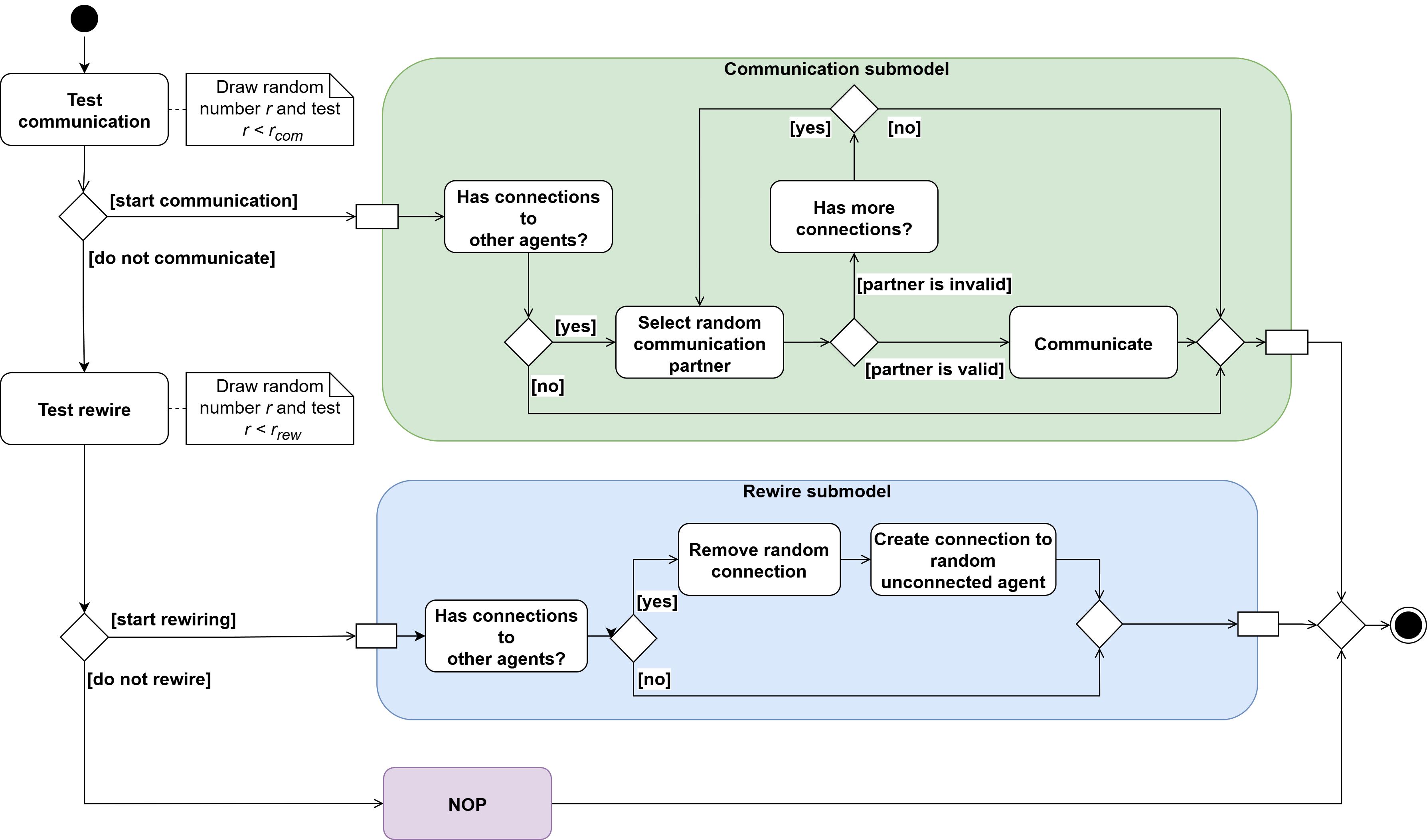
Communication serves two purposes. Agents gather interest about the innovation based on the interest status of their communication partner. For this, the model is parameterized with a set of numbers that indicate how many interest points their communication partner receives from interaction with them. Usually, agents gather the most interest through interaction with adopters, followed by interested agents, with aware agents generating the least amount of points. The interest points are gathered from every interaction with another agent. While concerning information of another quality, this is conceptually similar to (Macal et al. 2014). To initiate communication, the active agent searches for a valid communication partner from their social network, i.e. those who have performed no action in the current time step.

Furthermore, agent attitudes (environmental attitude and innovativeness) can be influenced by the other agent based on the relative agreement algorithm (Deffuant et al. 2002), as also done in Rai & Robinson (2015) and Sundaram et al. (2024). In this, the attitude \(x_{i}\) of agent \(i\) changes proportionally relative to the attitude \(x_{\hat{i}}\) of agent \(\hat{i}\) by the overlap \(min(x_{\hat{i}}+u_{\hat{i}}, x_{i}+u_{i})-max(x_{\hat{i}}-u_{\hat{i}}, x_{i}-u_{i})\) between the agreement, divided by an agent variable coined uncertainty \(u_{i}\), representing how strongly their attitude can be influenced by other agents. With asymmetrical uncertainties, this can differ between the two agents (Deffuant et al. 2002). Extremists in this model are agents at the extremes of the opinion distribution and low uncertainty. They are constructed by taking a set fraction of the population with the most extreme believes (at both ends of the spectrum) and assigning them a low uncertainty. In addition to this regular opinion dynamics, the model also allows for adaptations of this mechanic based on the difference of agreement of the agents. If this difference is smaller than the agreement threshold \(AGT\), the standard algorithm (as explained above) is applied. Otherwise, a (weighted) random event is drawn. With probability convergence, the standard algorithm is performed. With probability neutral, the attitude is not adjusted and with probability divergence, the inverse relative agreement algorithm is applied. For more details, see Abitz et al. (2024). The influence of other agents on the adoption is thus two-fold: by building interest, the interaction supports agents in reaching the interest threshold, a barrier that prevents adoption for agents with insufficient interest in the technology. Additionally, it influences the environmental attitude and the innovation of the agent, directly impacting the partial utility for these two decision factors.

Finally, agents have a chance to adapt their social network. In every time-step that agents don’t communicate, they might rewire their subjective network (with a probability of \(r_{rew}\)). If they do, they choose a random agent in their social network and remove the link. In exchange, a new link is created from this agent to another agent in the social network that they were not connected to before modifying links, based on their affinity.

Decision process and process plan

PVact is a dynamic model where agents’ variables can change in every time step. Along with numerous variables specific to the different submodels, agents have a state variable that represents their adoption status and phase within the decision process.

As households are comprised of humans, agents underlie bounded rationality assumptions. This is caught by the belief-desire-intention (BDI) model (Bratman 1999) with a high level of abstraction through the core characteristics of beliefs, goals or desires and intentions. Norling (2004) extended this abstraction by introducing elements taken from folk psychology ("how people think they think"). In PVact, belief is realized through the knowledge of agents about themselves, rooftop PV systems and their environment. As in IRPact (Johanning et al. 2020), desire is realized through the need to adopt. The intention is operationalized through the process model. The agents thus intend to act as they believe how they can achieve their goals based on their beliefs about the world (Norling 2004). The process model is a blueprint for the individual agent processes realized through the so-called process plan (idea of ‘plans as recipes’ as phrased in Norling (2004)). The process plan is a technical tool for the BDI model to specify the plans and actions of agents which is tightly interlinked with the process model, as it drives the agents to progress to the next step.

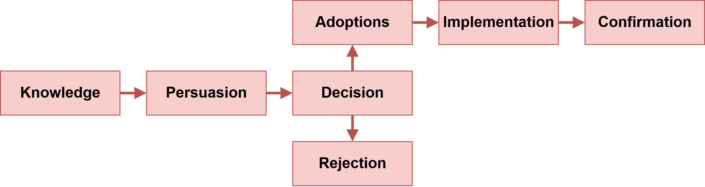
Similarly to Macal et al. (2014), the model is based on the theory of Diffusion of Innovation. The process model focuses on the persuasion and decision steps in the decision process model of Rogers (2003), which represent gathering information and interest about the technology (the persuasion step in Rogers (2003)) and taking the decision to accept or reject the innovation (the decision step in Rogers 2003), see Figure 2. In PVact, these phases are called the awareness phase (agents that are aware of the product gather information and interest) and the evaluation phase, in which the agents evaluate the technology in order to make a decision.

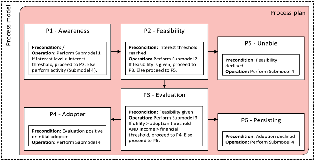
In the awareness phase, agents gather interest and information about the innovation by communicating with other agents (see above). The generated interest is then compared to an exogeneous variable (interest threshold). When sufficient interest is reached, agents transition to the next phase. As a pre-requisite for the decision to adopt, agents need to have the decision authority over the rooftop, which is operationalized by the assumption to live in a (semi-)detached house that is privately owned. This pre-requisite is checked in the feasibility phase following the awareness phase. If feasibility is not given, agents transition to the Unable phase, otherwise they shift to the evaluation phase.

In the evaluation phase, similarly to Macal et al. (2014), Nurwidiana et al. (2022), Palmer et al. (2015), Rai & Robinson (2015), Sundaram et al. (2024) and Wang et al. (2018), agents determine the utility of the PV system and compare it to a set threshold (adoption threshold). They furthermore check the household income against another threshold, the financial threshold, which impedes adoption for lower-income households (Macal et al. 2014; Nurwidiana et al. 2022). If agents decide against adoption or do not dispose of sufficient income, they transition to the Persisting phase, which allows for re-evaluation at a later time. If both conditions hold, agents transition to the Adoption phase. The phases and their transitions are shown in Figure 3.

In all non-transition phases (awareness, unable, persisting, adoption), agents can act conditionally. Based on the parameters \(r_{com}\) and \(r_{rew}\), agents can engage in communication with other agents (\(r_{com}\)) or form a new link in the social network (\(r_{rew}\)) as described above. In addition to this, several processes happen throughout the model; at the beginning of a simulation year, the techno-economic data is updated to reflect the respective data point from the time series (as in ). Then all agents in the persisting phase are moved to the evaluation phase and thus prompted to re-evaluate. The middle of the year (just before time step 27) sees two actions. First, renovation and construction events take place. For this, every agent who didn’t adopt yet gets to move to a single family house (construction) with probability \(r^{t}_{const}\) and evaluate straight away (Moglia et al. 2022). With a probability of \(r^{t}_{reno}\), agents living in (semi-)detached houses trigger a renovation event, which moves them straight to the evaluation phase. This is based on the assumption that these are occasions where households consult extensively with stakeholders that often also discuss energetic renovation options, such as rooftop PV. This assumption was based on insight from focus group research. This has been adopted in the revision.

Finally, the environmental attitude is updated for each agent, as described in paragraph 1.15. At the end of the year, all agents in the persisting phase are moved to the evaluation phase.

The decision process itself is comprised of five components. Agents evaluate the innovation based on its financial utility, social and local pressure and their environmental attitude and innovativeness. Their partial utilities are added based on five model parameters representing these partial weights. While the attitudes change over time (based on communication and a linear increase in the case of the environmental attitude), they are primarily determined by the set parameters. Social and local pressure are determined as the fraction of actual adopters among potential adopters in the perceivable environment of the agent. For social pressure, the connected agents in the social network, i.e. they have incoming or outgoing edges towards, are used (see Equation 2), for local pressure all agents within a 500 meter radius (determined with the haversine function) are considered (Equation 3), differing from van der Kam et al. (2024), Moglia et al. (2022) and Zhang et al. (2014) in implementation, but acknowledging the importance of spatial pressure. Similarly, the implementation of social pressure differs from Grant & Hicks (2020), Moglia et al. (2022), Palmer et al. (2015) and Wang et al. (2018), but agrees with their assessment of relevance.

\[\begin{aligned} U_{soc}(i)=\frac{\text{Actual adopters}_{social}}{\text{Potential adopters}_{social}}\end{aligned}\]

\[(2)\]

\[\begin{aligned} U_{loc}(i)=\frac{\text{Actual adopters}_{spatial}}{\text{Potential adopters}_{spatial}}\end{aligned}\]

\[(3)\]

Finally, inspired by prospect theory (Kahneman & Tversky 1979), financial utility is determined based on the difference of the net present value \(NPV(t_0, E(t_0, roof_{i}(i), roof_{o}(i)))\) of a PV system with a yearly yield of \(E(t_0, roof_{i}(i), roof_{o}(i))\) (see Equation 1) relative to an average system. The NPV is determined based on investment cost, collected revenue from feed-in and avoided cost over a 20 year period, as shown in Equation 4:

\[\begin{aligned} NPV(t_0, E(t_0, roof_{i}(i), roof_{o}(i)))= & \nonumber -p_{invest}(t_0) + \\ & \nonumber \sum_{t=0}^{t_{FIT}=20} \left( \frac{1}{(1+r_{int}(t_0))^t} * (FIT(t_0)*(1-SC)) \right. + \\ & \Bigl. p_{elec}(t_0)*(1+p_{esc})^t*SC*E(t_0, roof_{i}(i), roof_{o}(i)) \Bigr)\end{aligned}\]

\[(4)\]

\(p_{invest}(t_{0})\) is the investment cost of the PV system at time \(t_{0}\), \(FIT(t_{0})\) is the guaranteed feed-in-tariff, \(SC\) is the self-consumption coefficient (how much of the generated electricity the household consumes itself), \(p_{elec}(t_{0})\) the electricity price and \(r_{int}(t_{0})\) the interest rate. While all cost are determined for the time of decision \(t_{0}\), time-variable components are assumed to progress, e.g. with \(p_{esc}\) in the case of electricity prices.

In order to make the NPV consistent with other agent decision variables⁸ as the financial utility, it is normalized and scaled logistically using a symmetrical function before the result is normalized again. The first step in this is determining the normalized NPV \(NPV_{norm}\) (see Equation 5):

\[\begin{aligned} NPV(t_0, E(t_0, roof_{i}(i), roof_{o}(i)))_{norm} = \frac{NPV(t_0, E(t_0, roof_{i}(i), roof_{o}(i))) - NPV_{min}}{NPV_{max} - NPV_{min}}\end{aligned}\]

\[(5)\]

\(NPV_{min}\) and \(NPV_{max}\) are the min/max NPV values across the years 2008 to 2019 over all potential combinations of inclinations and orientations. This normed NPV is then transformed into logistic form according to Equation 6:

\[\begin{aligned} NPV(t_0, E(t_0, roof_{i}(i), roof_{o}(i)))_{logistic} = \frac{1}{1+e^{(-1*(NPV(t_0, E(t_0, roof_{i}(i), roof_{o}(i)))_{norm} - 0.5))}}\end{aligned}\]

\[(6)\]

In the final step, \(NPV(t_0, E(t_0, roof_{i}(i), roof_{o}(i)))_{logistic}\) is rearranged to \([0, 1]\) to correspond to the financial utility \(U_{f}(i)\), as shown in Equation 7. This is done as the logistic function for the NPV only yields values within a limited subinterval of the unit interval for actual rooftops in the case studies.

\[\begin{aligned} U_{f}(i) = \frac{NPV(t_0, E(t_0, roof_{i}(i), roof_{o}(i)))_{logistic} - logistic_{0}}{logistic_{1} - logistic_{0}}\end{aligned}\]

\[(7)\]

with \(logistic_{1}\) and \(logistic_{0}\) being the maximum and minimum value of the logistic NPV respectively. Thus, a financial utility of 0 means that the PV system is among the worst performing in the model, whereas a utility of 1 evaluates it as among the most monetarily favorable. The financial utility is centered among average systems with a value of \(0.5\) and, depending on the makeup of the case study, even a negative NPV could evaluate to a value \(> 0\). We chose not to use this as a barrier, since households might still adopt rooftop PV due to other factors, as shown in empirical studies. Instead, PVact features a financial threshold oriented on the households purchase power, which prevents households from adopting if their purchase power \(PP_{i}\) is below this threshold.

The factors determining the utility of the PV system are added as weighted factors. Weights can be set arbitrarily as long as they accumulate to unity⁹, but for the base scenario were set based on linear regression of a large-scale survey (Nurwidiana et al. 2022, van der Kam et al. 2024). Finally, the model features two (further or main) free parameters: the adoption threshold \(AT\) determines which utility has to be met or exceeded during the evaluation in order for agents to adopt, while the interest threshold \(IT\) is used to move agents from the interest to the feasibility phase (see above).

The adoption threshold is then used in the evaluation phase for the decision for or against adoption, together with the financial threshold mentioned above. Similarly to Macal et al. (2014), Palmer et al. (2015), Sundaram et al. (2024) and Wang et al. (2018), the partial utility sum needs to exceed the threshold in order to consider adoption. The decision for adoption of agent \(i\) in timestep \(t\) is thus Equationted according to Equation 8:

\[\begin{aligned} state(i)^{t+1} = \begin{cases} P4, & w_{fin} * U_{f}(i) + w_{soc} * U_{soc}(i) + w_{loc} * U_{loc}(i) + \\ & w_{env} * ec(i) + w_{ino} * in(i) \geq AT\, \& \,PP(i) \geq FT \\ P6, & else \end{cases}\end{aligned}\]

\[(8)\]

The state of agent \(i\) at the next time step \(t+1\) is thus determined by the evaluation of the systems utility and their purchase power \(PP(i)\) relative to the financial threshold \(FT\).

Initialization procedure

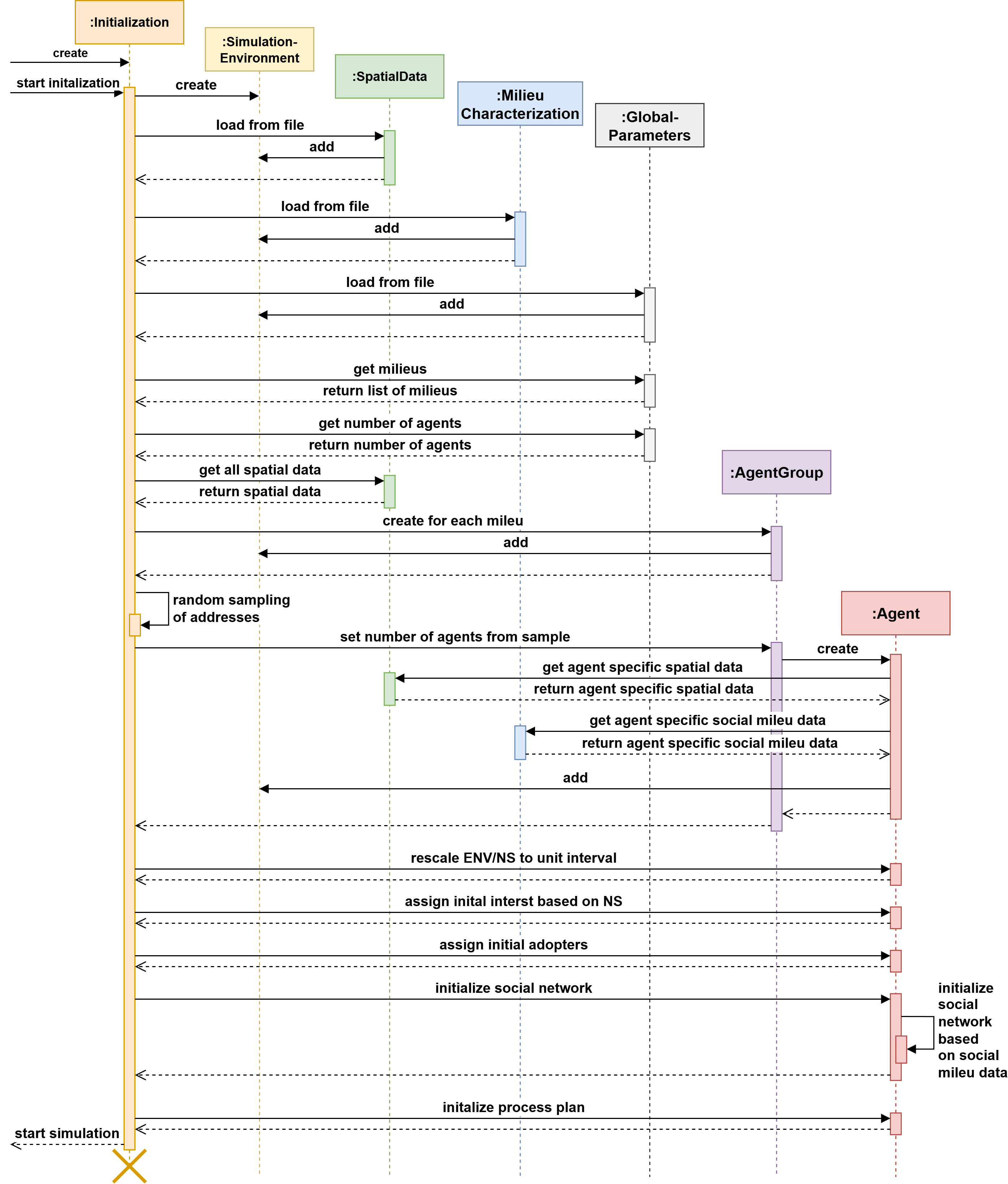
The aspects mentioned so far can be found in the initialization process within PVact. The overall process is modeled in Figure 4. All components and data within PVact are held within a simulation environment. The environment object allows agents to access the knowledge during simulation. In the first step during initialization, this environment object is created. It is a prerequisite for the social, spatio-economic and attitudinal data loaded from files in the following steps. In addition to agent-specific parameters, global simulation-related data, such as the level of detail of log output or the number of agents, are also loaded. Following the import of all external files, the agent initialization begins by preparing the agent groups. In PVact, agents are not created directly but are derived from groups. These groups are based on the Sinus milieus. Agents derived from the same group share similarities in terms of parameterization and behavior.

Methodology

Modeling allows to formalize informal ideas through mathematical symbols or code, disambiguating otherwise vague concepts (Edmonds et al. 2019). Computer modeling for policy analysis, however, is troubled by confusion about modeling (Bankes 1993) and underspecification of the models’ purpose in social simulation, which in turn influences model building, judgement, justification, checking, validation and verification (Edmonds et al. 2019).

Edmonds et al. (2019) argue to present models as purpose-specific tools and warn of using explanatory models for under-explored contexts as this tends to lead to explaining a system by any way that allows to model a system a certain way or a good data fit (Edmonds et al. 2019). Explanatory models are imperative for understanding where predictive models can be employed successfully, but require a causal chain from set-up to consequences. Beyond a good understanding of the modeled context, predictive models require experimental validation (Bankes 1993; Bankes et al. 2013), extensive knowledge, resolvable (linear) uncertainties, accurate measurements and mature theory (Bankes 1993; Bankes et al. 2002)¹⁰. They are furthermore unreliable for deeply uncertain contexts and require closed boundaries, which makes them very challenging for policy modeling, which is characterized by complex and uncertain problems.

For problem with deep uncertainty, predictive modeling is thus misleading (Kwakkel 2017) and a different approach is required. Instead of a singular representation of the modeled phenomenon, exploratory modeling investigates a range (coined an ensemble) of plausible models (Bankes 1993), based on observed uncertainty of the problem and constrained by existing knowledge and data (Bankes et al. 2013). In contrast to predictive modeling, uncertainty is increased instead of avoided. This is understood from the perspective that many models are a plausible representation of the studied phenomenon (Bankes 1993) and models that are consistent with the data they can explain are not unique and data is compatible with a range of models (Bankes et al. 2013). Bankes et al. (2002) recommend to do experimentation by agile interaction between researchers and software, as humans are superior at pattern interpretation based on pragmatic and tacit knowledge. Through highly interactive research, collaborative conclusions can be reached through interactive mechanisms. Model exploration is done by a number of computation experiments over an ensemble of scenarios differing in their parameterization, looking for ‘interesting guesses’ on the basis of sampling plausible model inputs (Bankes 1993). Thus, policy decisions can be supported even where approaches such as optimization or predictive modeling is not applicable (Bankes et al. 2013).

Overall, exploratory modeling can be described as a methodology for sampling a parameter (sub-)space characterized by uncertainty to interactively explore the model behavior over an ensemble of scenarios and possible worlds within an experimental context. Exploratory modeling is close to the concept of theoretical exposition in Edmonds et al. (2019), which focuses on the exploration of the consequence of assumptions and model mechanisms that require exploration and assumes that the behavior of the system is represented by a full set of simulation outcomes over all initialization. It is thus in line with the ensemble approach seen with exploratory modeling above. While it can be used to test hypothesis about how the model mechanisms work, it can also be employed to compare assumptions and investigating the change in simulation outcome for these cases (Edmonds et al. 2019). The authors warn of mistaking the model behavior with the behavior of the modeled system and state that it should not claim anything about it as it doesn’t lend empirical support to derived claims. This approach is very much in line with exploratory modeling and lends methodological credibility to it; however, it requires extensive testing of the model. Both the code for the framework IRPact was tested throughout development (internal validation) and the model was tested through a range of static and dynamics tests on related toy models (theoretical validation).

Due to the complex social nature of residential rooftop PV adoption and the complexities shown in (Johanning et al. 2022, 2023), exploratory modeling and theoretical exposition seemed to be the most appropriate approach for addressing the research question. As the research question was interested in the relative importance of the different weights of the model, variation of the weights seemed an important factor in constructing the model ensembles to investigate. Other factors of interest were opinion dynamics, normative pressure and network structure. The research is guided interactively, with a rough survey of the scenarios being followed by iteratively adding more detailed simulation runs to the parameter landscape in order to get a more informed and granular image of the observed parameters, addressing the interactiveness of exploratory research. Exploration follows conventional scenario discovery as a three step process including generation (sampling from input parameter space), identification (output reduction to one single value) and rule induction (identification of interesting parameter regions), as sketched in Steinmann et al. (2020). For this, the input parameter space was varied by the adoption threshold based on fixed scenarios laid out below (generation). The rich output of the models, with yearly varying multiple dimensions for each agent was reduced to the cumulative adoption throughout the whole system (identification). Finally, the parameter region where large dynamics were seen was investigated more granularly (rule induction). Furthermore, this paper followed a more classical approach by focusing on outcome comparison with respect to Steinmann et al. (2020), except in scenario family 1 (see below) where dynamics over time were also addressed in order to keep the research scoped and to get a rough overview of the parameter landscapes. In line with Bankes et al. (2002), which views the ideal setup as representing the phenomological level in the model code and leaving analytical manipulation to be done in the experimental context, this research is done with the IRPact framework in an experimental context that separates the model execution (IRPact) from the simulation execution infrastructure.

Operationalization of explorative modeling

Exploratory modeling requires the investigation of a whole ensemble of models to cover the variety of assumptions and uncertainties featured in complex social computer models. It designs a range of computational experiments with different parameterization that are seen as scenarios or strongly relate to scenarios (e.g., as subspaces), with a particular focus on invariants or properties of (sub-)sets of model instances. Eventually, explorative models serve to inform robust adaptive policies that are built on model ensembles. Methodologically, the approach involves interaction between the researcher and the ensemble investigation within experimental contexts. Together, these aspects constitute the four concepts (ensembles, adaptive policies, interactiveness and experimental contexts) that Bankes et al. (2002) identified.

Due to the complex social nature of residential rooftop PV adoption and the complexities shown in Johanning et al. (2023) and Johanning et al. (2022), exploratory modeling seems to be the most appropriate approach for addressing the research question. As the research question is interested in the relative importance of the different weights of the model, variation of the weights appears to be an important factor in constructing the model ensembles to investigate. Other factors of interest are normative pressure, opinion dynamics and network structure. The design of the ensembles with a particular focus on these factors is addressed below in Section 2.11. The research is guided interactively, with a rough survey of the scenarios being followed by iteratively adding more detailed simulation runs to the parameter landscape in order to get a more informed and granular image of the observed parameters, addressing the interactiveness of exploratory research. This research is done with the IRPact framework in an experimental context that separates the model execution (IRPact) from the simulation execution infrastructure detailed in Section 2.19 below. This was done in line with Bankes et al. (2002), which views the ideal setup as representing the phenomological level in the model code and leaving analytical manipulation to be done in the experimental context (i.e., the software environment).

The only remaining element of exploratory modeling that was not addressed in this research methodology are adaptive policies. As the focus of this research lies on exploring the parameter ensemble connected with the importance of decision factors, the policy level would have added another layer on the investigation. In order to translate policy options to the models, a solid understanding of the model ensemble would be necessary, as it would otherwise not be clear which behavior would be attributed to the decision factors and the (direct) interactions of the agents themselves and to the investigated policy. As this article follows the model-driven approach noted in Bankes (1993), the research question focuses on an investigation of the properties of this class of models rather than comparing model results to observed data or investigating policy questions, as Bankes (1993) noted that parameter selection should depend on the investigated research question. The focus was put on the identification of chaotic and stable regions that are subsequently required for Exploratory Modeling and Analysis to investigate what policies these regions support (Bankes et al. 2013). In summary, the investigation of (adaptive) policies was decided to be done in subsequent research.

Steinmann et al. (2020) describes conventional scenario discovery as a three step process including generation (sampling from input parameter space), identification (output reduction to one single value) and rule induction (identification of interesting parameter regions). For this, the input parameter space is varied by the adoption threshold based on fixed scenarios laid out below (generation). The rich output of the models, with yearly varying multiple dimensions for each agent is reduced to the cumulative adoption throughout the whole system (identification). Finally, the parameter region where large dynamics are seen is investigated more granularly (rule induction). Furthermore, this article followed a more classical approach by focusing on outcome comparison with respect to Steinmann et al. (2020), except in scenario family 1 (see below) where dynamics over time were also addressed. This was done to keep the paper scoped and to get a rough overview of the parameter landscapes; this was by no means intended to fully understand the model landscape, but to serve as a starting point for future explorations.

Through the methodological design described above, this article brings together the requirements, assumptions and constraints of a theoretical exposition with the principles and methods of exploratory modeling.

Scenario design

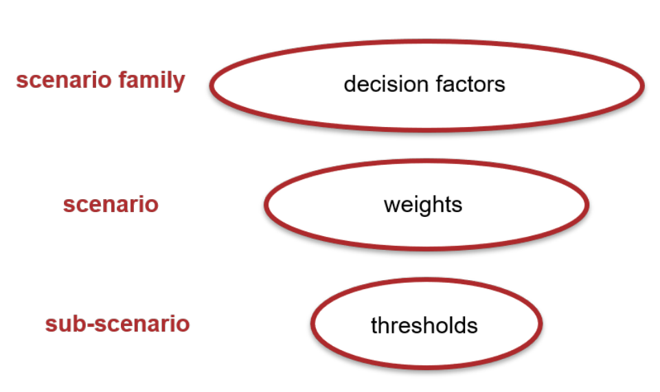
In addition to the technical environment, the experimental setup includes the sampling strategy. The sampling strategy in this research is to investigate different decision factors (through sets of scenario families), with the variation of the core parameter adoption threshold (see Section 1.53) within each scenario as defined by the weights and the idiosyncracies of the scenario family. The sampling strategy is thus hierarchical, with the scenario family determining the influencing factors, the scenarios specifying their weights and sub-scenarios altering the adoption threshold, as visualized in Figure 5. Using the terms laid out in Bankes et al. (2013), the exploration thus is done over real-valued parameters.

Sceanario family 1 builds on Johanning et al. (2023) and investigates financial performance and normative pressure, while the other scenarios focus on agent attitudes (specifically environmental attitude and innovativeness). Scenario family 2 represents the influence of these attitudes and the financial evaluation without opinion dynamics, while scenario family 3 investigates them with paying attention to opinion dynamics.

All scenarios use a combination of three decision factors in their decision making process (monetary evaluation, local peer pressure and social peer pressure in scenario 1, monetary evaluation, environmental attitude and innovativeness in scenarios 2 and 3) that corresponds to the weights used in the decision phase within the model. As noted in Section 1.53, these weights add to 1. In order to sample the parameter space in these scenarios, the weights were chosen as depicted in Figure 6, with the addition of the case where \(w_{fin} = 0.75\) and the weights of the other two factors correspond to 0.125. The choice of the decision factors to investigate were based on the mentioned empirical and theoretical work that stresses the importance of monetary factors, attitudes and social pressure.

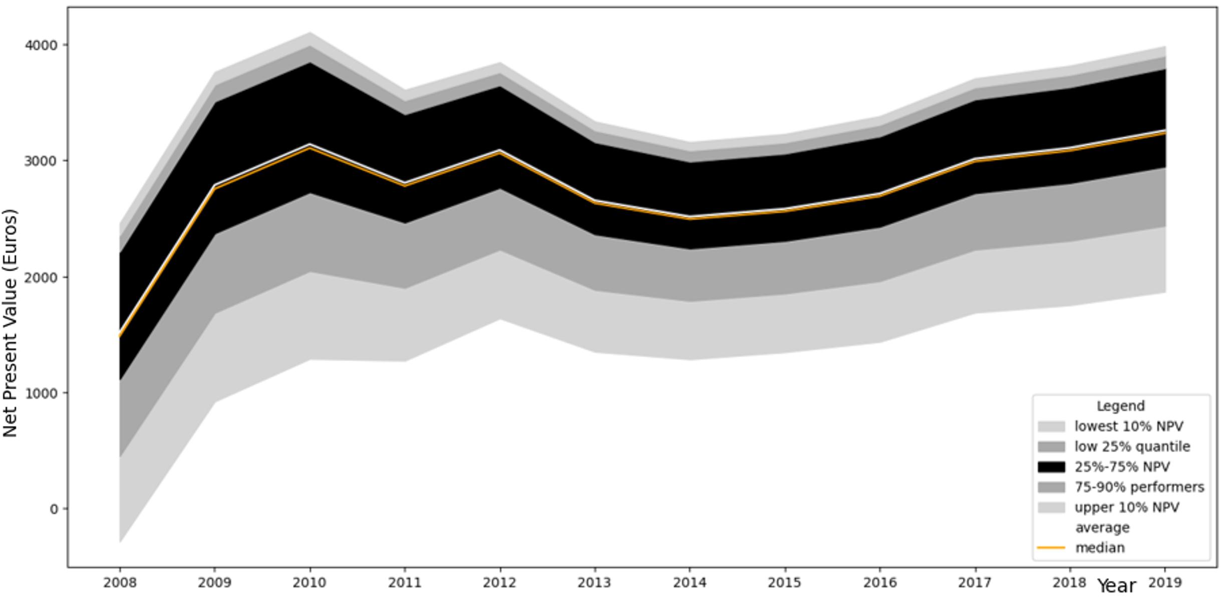
The investigation uses data from the case study of the city of Leipzig (Germany) which focuses on the spatio-granular adoption of rooftop PV by agents living in (semi-)detached houses within the timeframe of 2008 – 2019 (see also Scheller et al. 2022). As described in Section 1.40, their attitudes are individual parameters/attributes and the normative pressure is determined by the fraction of adopters within a local area of 500 meters around the agent (local pressure) or in their individual social network (social pressure). The financial evaluation uses a logit-based transformation of the individual agents’ net present value (NPV) against reference NPVs in order to scale the partial utility to the unit interval. The progression of the NPVs of throughout the simulation years is shown Figure 7.

Scenario Family 1

Scenario family 1 focuses on the financial performance and normative pressure as decision drivers of households. For this, monetary evaluation, local pressure and social pressure were chosen as decision factors that were investigated with different weights throughout different sub-scenarios (all other decision factors were weighted with 0). For this, the behavior of the decision factors in isolation is analyzed before the system behavior under their combination is investigated. The analyzed scenarios are (with the notation of monetary pressure - social pressure - local pressure): 0-1-0, 0-0-1, 0.5-0-0.5, 0.5-0.5-0, 0-0.5-0.5, 0.5-0.25-0.25, 0.25-0.5-0.25, 0.25-0.25-0.5, 0.75-0.125-0.125, 0.125-0.75-0.125, 0.125-0.125-0.75 and 0.33-0.33-0.33¹¹.

Scenario family 2

Scenario family 2 looks at the interplay of monetary evaluation and household attitudes without the use of opinion dynamics. Social pressure is thus ignored and the analyzed scenarios are (with the notation of monetary pressure - environmental attitude - innovativeness): 0-1-0, 0-0-1, 0.5-0-0.5, 0.5-0.5-0, 0-0.5-0.5, 0.25-0.5-0.25, 0.25-0.25-0.5, 0.75-0.125-0.125 and 0.33-0.33-0.33. The scenario 1-0-0 has been discussed in scenario 1 already, which is why it is left out of this analysis.

Scenario family 3

The 3rd scenario family focuses on the influence of opinion dynamics in cases where the monetary evaluation and household attitudes influence adoption behavior. For these scenarios, core sub-scenarios from scenario family 2 are taken and the strength of opinion dynamics is varied to investigate the change of adoption patterns with altered behavior of opinion dynamics. For this, the parameters for the relative agreement algorithm are set differently according to the scenarios to observe how the strength of opinion dynamics changes the systematic adoption behavior (see Table 1).

For each of these cases, only a limited set of sub-scenarios with illustrative weights are used as support cases, namely 0-1-0, 0-0-1, 0.75-0.125-0.125 and 0.125-0.75-0.125, with the medium level of opinion dynamics also showing the cases 0.5-0-0.5, 0.5-0.5-0, 0-0.5-0.5, 0.25-0.5-0.25, 0.25-0.25-0.5, 0.125-0.125-0.75, 0.33-0.33-0.33.

Altering the opinion dynamics works in different ways; for some scenarios, the intensity of opinion dynamics were increased by strengthening convergence (scenarios IIIC-*) or divergence (scenarios IIID-*). To reduce the impact of opinion dynamics, parameters were also decreased to show less opinion dynamics (scenarios IIIO-*). Finally, the influence of extremists was investigated by increasing the proportion of extremists (scenarios IIIE-*). The parameters for the basic scenario family (III) and the variation of opinion dynamic parameters can be found in Table 1.

Table 1: Relevant opinion dynamic parameters for the scenarios in scenario family III-*.

Parameter	III	IIIC	IIIO	IIID	IIIE
attitude gap	0.1	0.9	0.03	0.9	0.1
probability convergence	0.25	0.75	0.1	0	0.25
probability divergence	0.25	0	0.1	0.75	0.25
probability neutral	0.5	0.25	0.8	0.25	0.5
speed of convergence	0.1	0.25	0.03	0.25	0.1
extremist parameter	0.125	0.125	0.125	0.125	0.75

Computational infrastructure

The calculations were executed at the high-performance computing cluster of the University Computing Center of Leipzig University. They used the ‘Paul’ general computing cluster featuring MegWare Saxonid nodes with 2 AMD(R) EPYC(R) 7713 @ 2.0GHz - Turbo 3.7GHz CPUs with 64 cores each, 512GB registered ECC DDR4@3200MHz RAM and a 25Gbit/s redundant Ethernet and 100GBit/s Infiniband compute node-storage-network. The simulations were done with a .jar-based build of the 1.0 release of IRPact (https://github.com/IRPsim/IRPact/)¹² from July 27th 2023, using slurm (https://slurm.schedmd.com/documentation.html)¹³ as workload manager. For each scenario, a dedicated input .json file was written, which was altered for the free parameters of investigation on a script basis. The script was also used for managing the simulation execution. For parameter regions where errors were encountered or where results required calculations with higher granularity, another set of simulations was scheduled and executed.

Results

Scenario I

Normative pressure only

For the scenarios I-0-1-0, I-0-0-1 where just normative pressure was considered for the adoption of an agent (i.e., that a certain fraction of agents related with the principal agent need to have adopted), very strong adoption patterns can be seen. Figure 8 shows the agent adoption behavior for these scenarios with different adoption thresholds (0.0185851 and 0.0185852 for scenario I-0-0-1 and 0.2 and 0.200000001 for I-0-1-0).

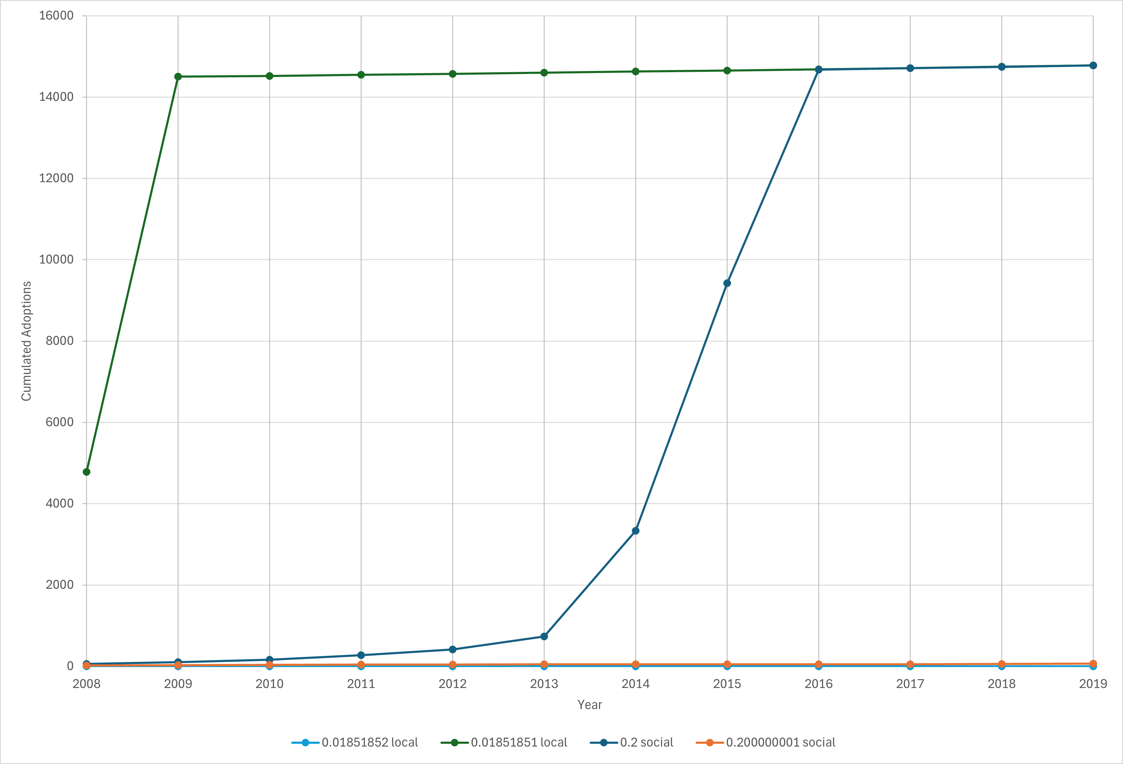
The results strikingly show how chaotic the system is if it is based solely on normative pressure. Both system configurations show very strong critical points (0.0185851 for local pressure and 0.2 for social pressure) which exhibit very strong adoption (all agents that can potentially adopt in the scenario); beyond these points, however, adoption patterns collapse immediately with a minor adjustment of the required utility for adopting, showing a critical point beyond which the adoption pattern collapses.

This effect can also be observed for the combination of both forms of normative pressure, albeit to a much smaller degree. In the case where equal weight is given to local and social pressure (scenario I-0-0.5-0.5), the change in adoption pattern is very strong still, but spread out over a wider band of adoption thresholds and somewhat more gradual (see Figure 9). Yet, the scenario shows that normative pressure (by itself) leads to strong runaway effects and shows the criticality of the system.

NPV only

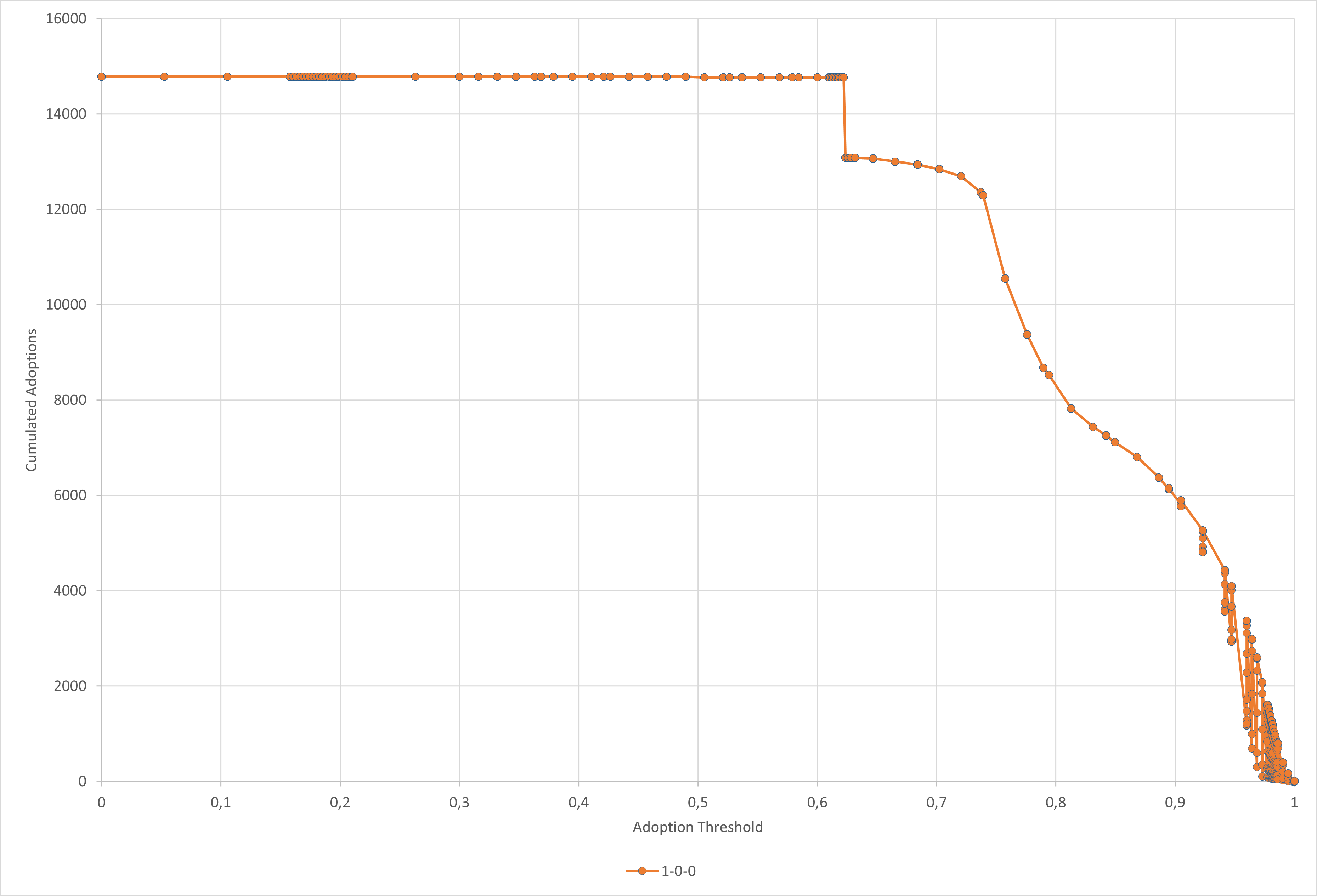
For the scenario I-1-0-0, a more gradual adoption decline curve is seen with increasing required utility for adoption. As shown in Figure 10, up to a required AT of 0.623, every agent who can adopt adopts, followed with a (semi-)plateau of  12,500 adoptions and a steady decline for the rest of the parameter region.

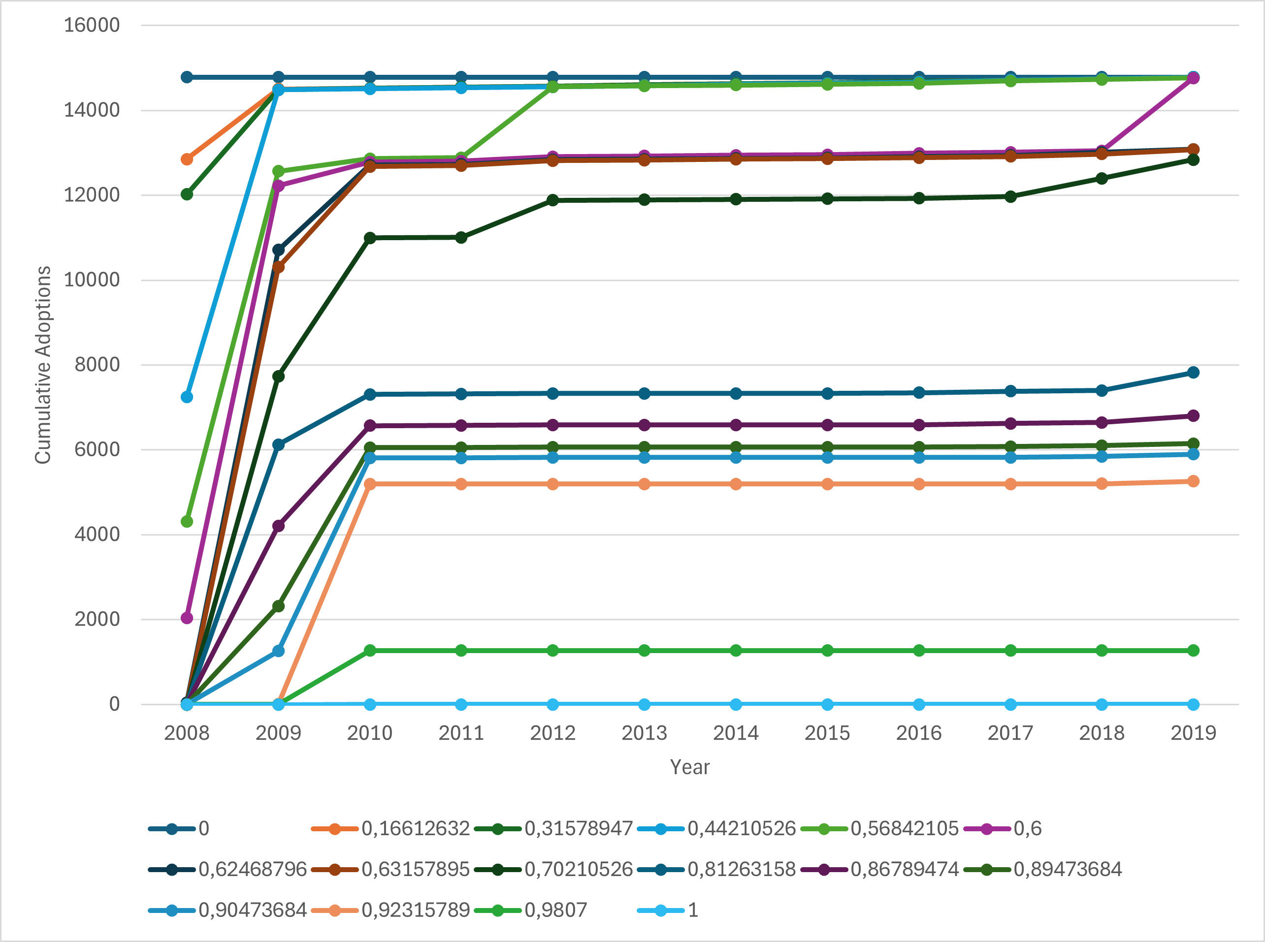
The same picture can be observed over time. Figure 11 shows the adoption patterns throughout the simulation horizon for different adoption thresholds. The graph show that for most of the simulation, the adoption occurs in the first years; due to the low NPV in the years 2008 and 2009 (see also Figure 11), for cases where a high NPV is required (i.e., high adoption threshold) adoption is delayed into years of a higher NPV (i.e., 2010).

The operationalization of the monetary evaluation thus shows a much more gradual distribution (for the higher parameter region) and seems to work as a moderating factor for the extreme behavior seen in the experiments just including the normative pressure. This suggests that the combination of the normative pressure and the financial evaluation might show interesting model behavior.

Interplay of normative pressure and monetary evaluation

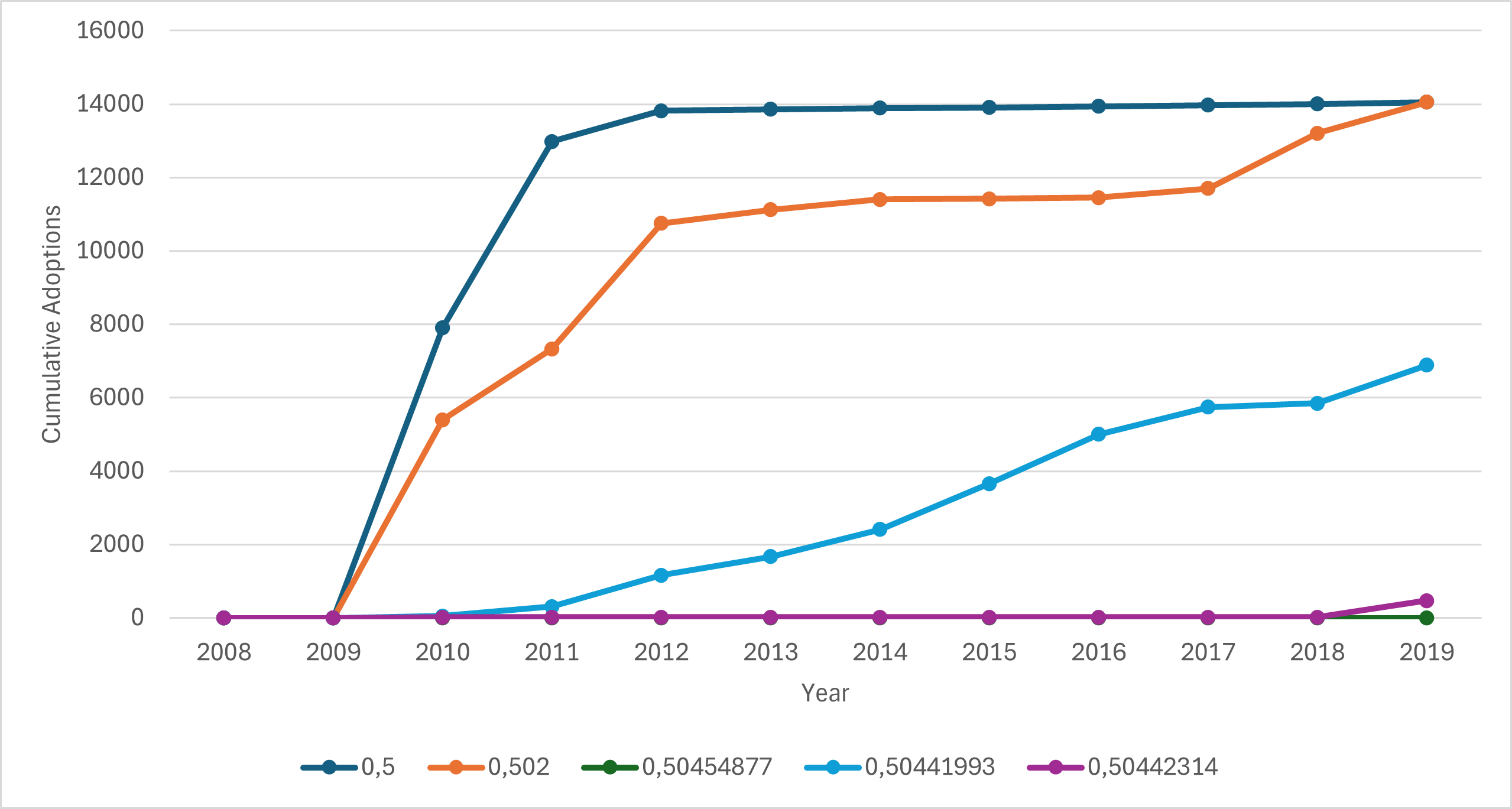
Similarly to the scenario I-0-0.5-0.5 described above, combining monetary evaluation and normative pressure shows adoption behavior that is very sensitive to the adoption threshold chosen. For the local case (scenario I-0.5-0-0.5), full adoption at the end of the simulation is seen with an adoption threshold of 0.502, whereas above 0.5045, no adoption is seen over the course of the simulation, as can be seen in Figure 12.

The picture is very similar in scenario I-0.5-0.5-0, where adoption depends solely on the monetary evaluation and social peer pressure. In this case, full adoption is seen up to a threshold of around 0.53, with little adoption around 0.54, which completely drops off at 0.578 (see Figure 13).

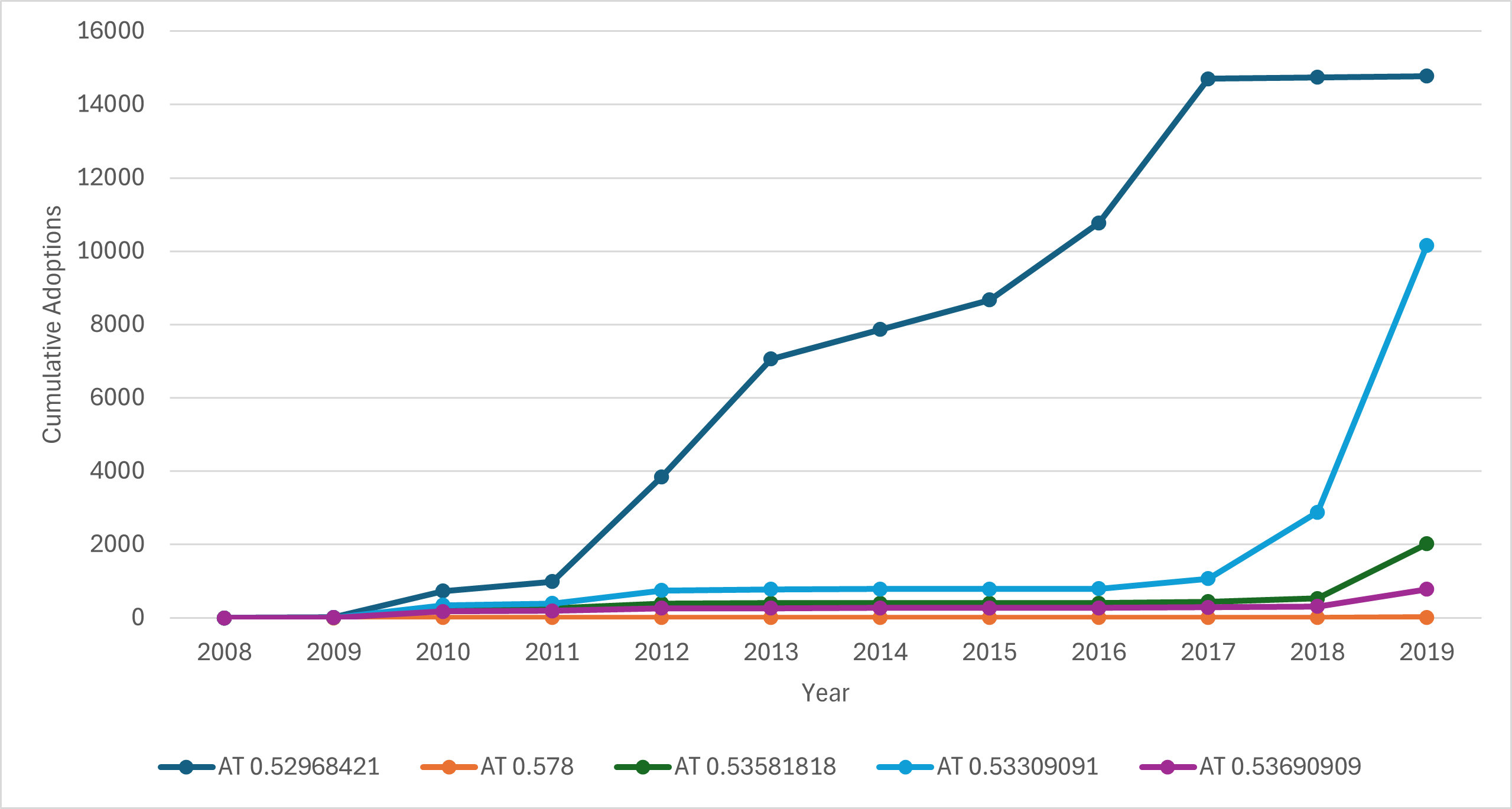
Again, the case of dependence on social peer pressure shows strong sensitivity to the adoption threshold, albeit in a wider parameter band than is the case for local pressure (i.e., scenario I-0.5-0-0.5).

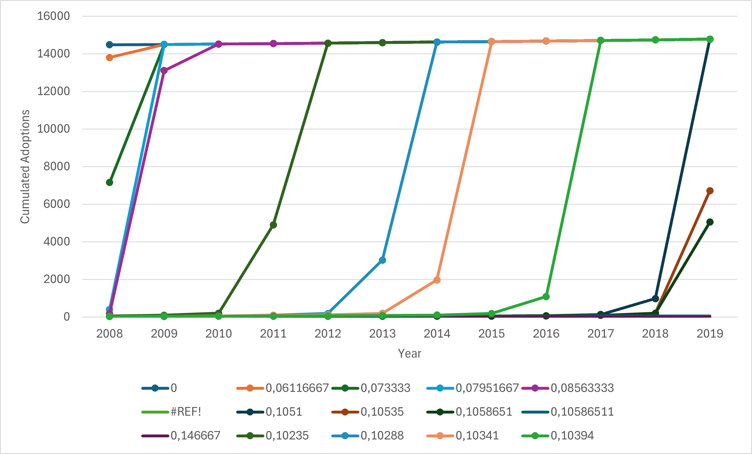
This steep decline in adoption behavior can be seen throughout the entire surveyed parameter landscape. With different parameter constellations, both the slope of the adoption decline through different parameters and the critical point shifts (i.e., at what adoption threshold the system tips from full adoption to a rapid decline in adoption) as can be seen in Figure 14. The strong sensitivity to the adoption threshold within very narrow bands appears to be a characteristic of the operationalization of normative pressure within the model.

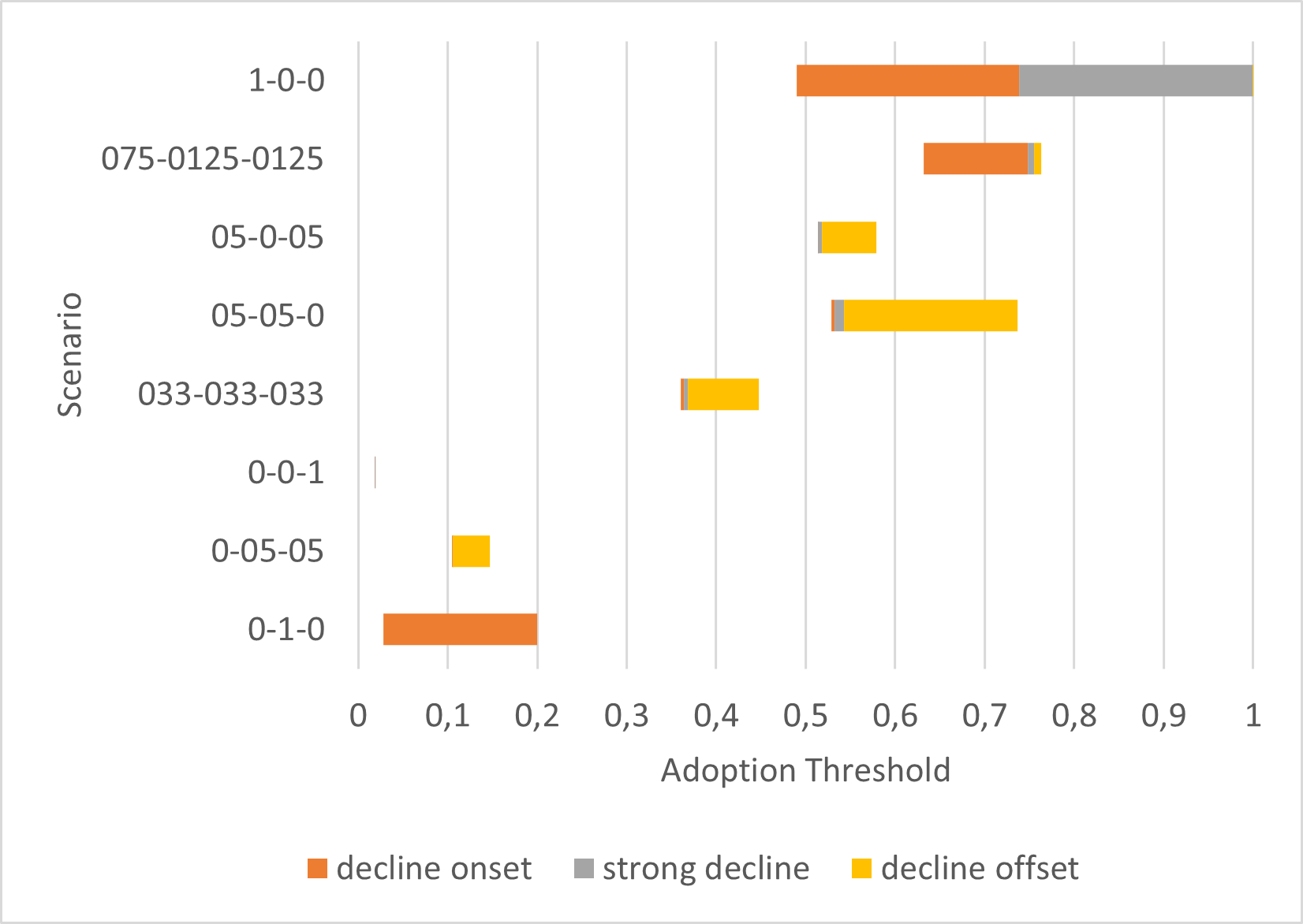
Overall, this model ensemble is characterized through steep adoption differences within narrow bands. This is particularly the case for models that are heavily focused on normative pressure. Monetary evaluation seems to be a somewhat moderating factor. This is also seen in Figure 15, which shows very narrow bands for the scenarios based on normative pressure and much wider sensitive parameter bands for scenarios focusing on monetary evaluation.

Scenario II

The scenarios within the second scenario family look at the interplay of monetary evaluation and household attitudes without the use of opinion dynamics. Attitudes thus are set in the initialization of the simulation and (with the exception of the linear increase of the environmental attitude described in II-C) remain constant throughout the simulation horizon.

The results of the attitude-based scenarios are much more gradual than is the case with normative pressure.

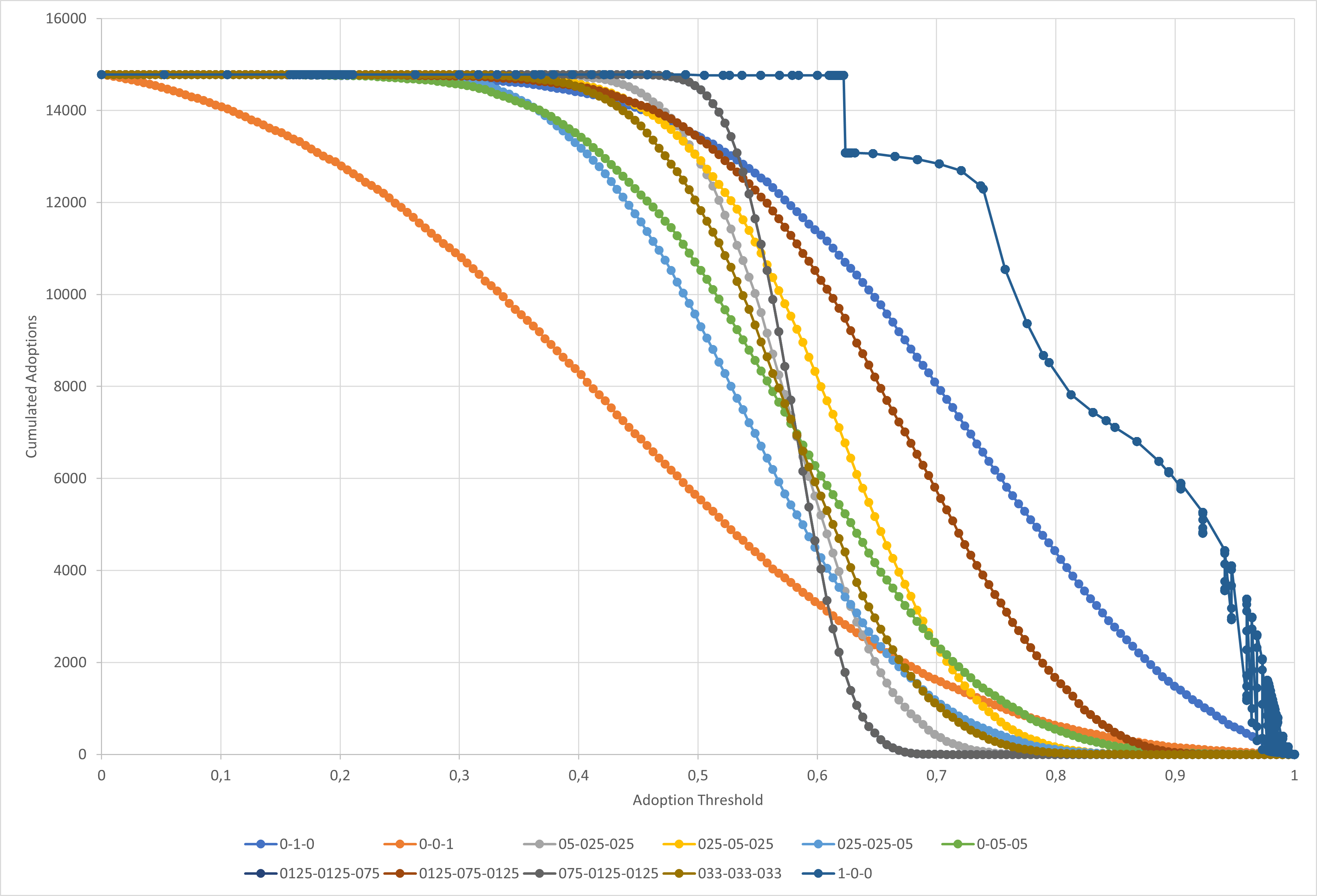
For most of the parameter (sub-)space of the adoption threshold, cumulated adoptions over the simulation period are situated between the scenario II-0-0-1, where adoption decisions are purely based on an agents’ innovativeness and II-0-1-0, where environmental awareness dictates whether agents adopt (see Figure 16). While in the case of innovativeness, the spread is wide and even a low adoption threshold leads to some agents not adopting, the drop where some agents don’t adopt over the simulation period in II-0-1-0 comes at a much later point. This can be explained by the linear increase of the environmental attitude throughout the simulation, contributing to the utility of the PV system. The case of the combination of these two attitudes (scenario II-0-05-05) shows the expected behavior for the largest parameter region, where it is situated between these two scenarios, showing the delayed onset of reduced adoption up to a threshold of 0.78, where adoptions are lower even than each single case.

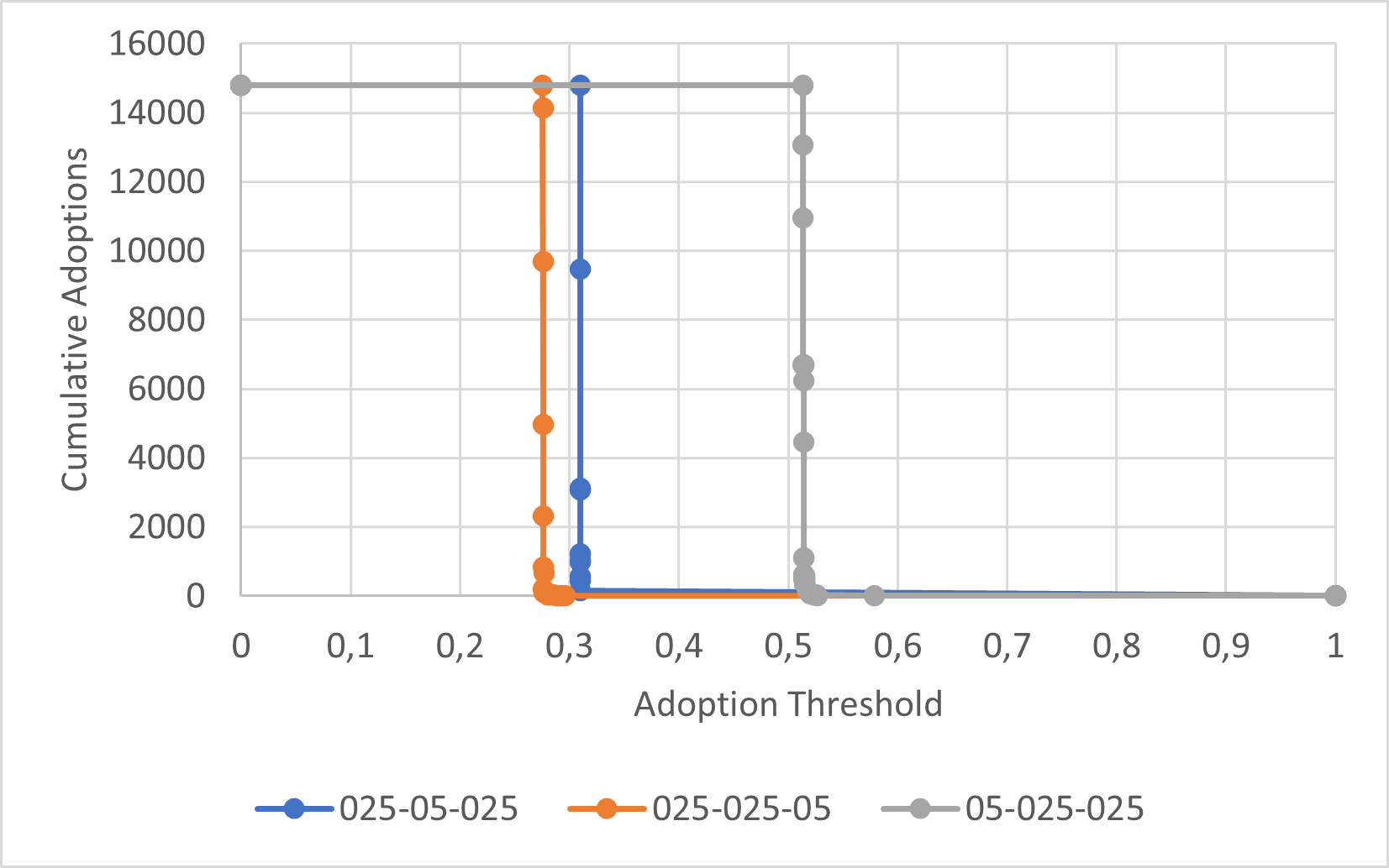
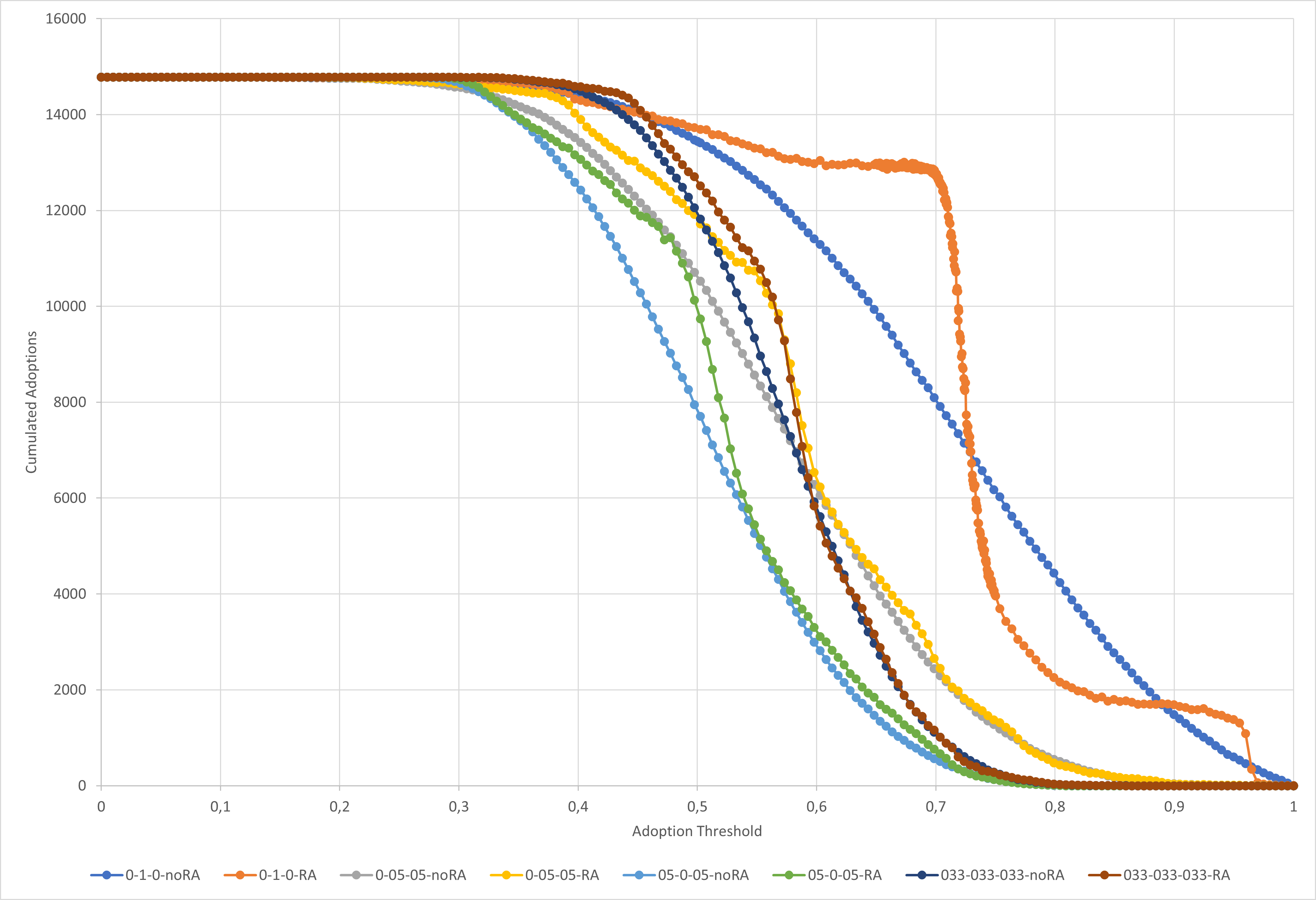
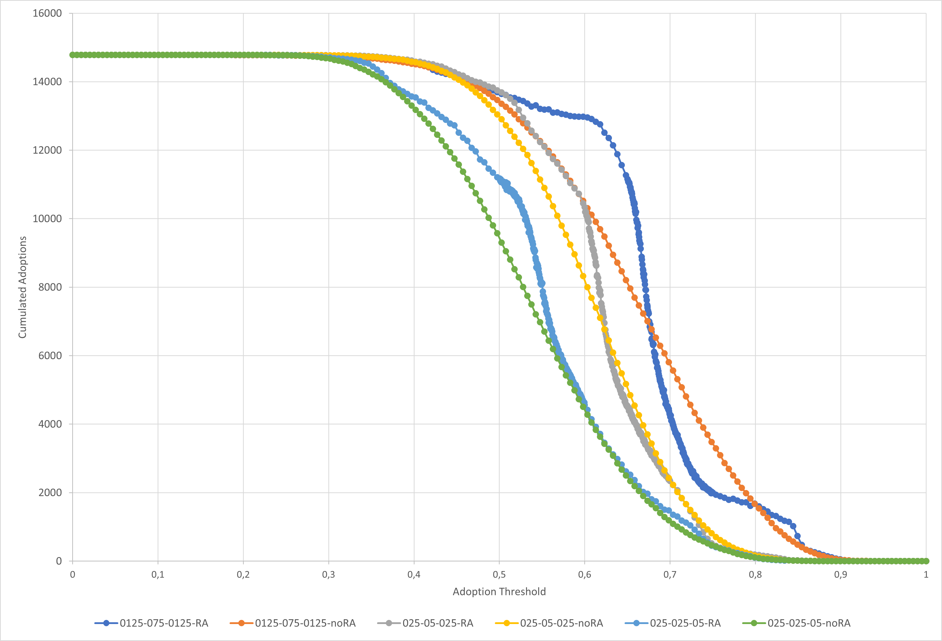
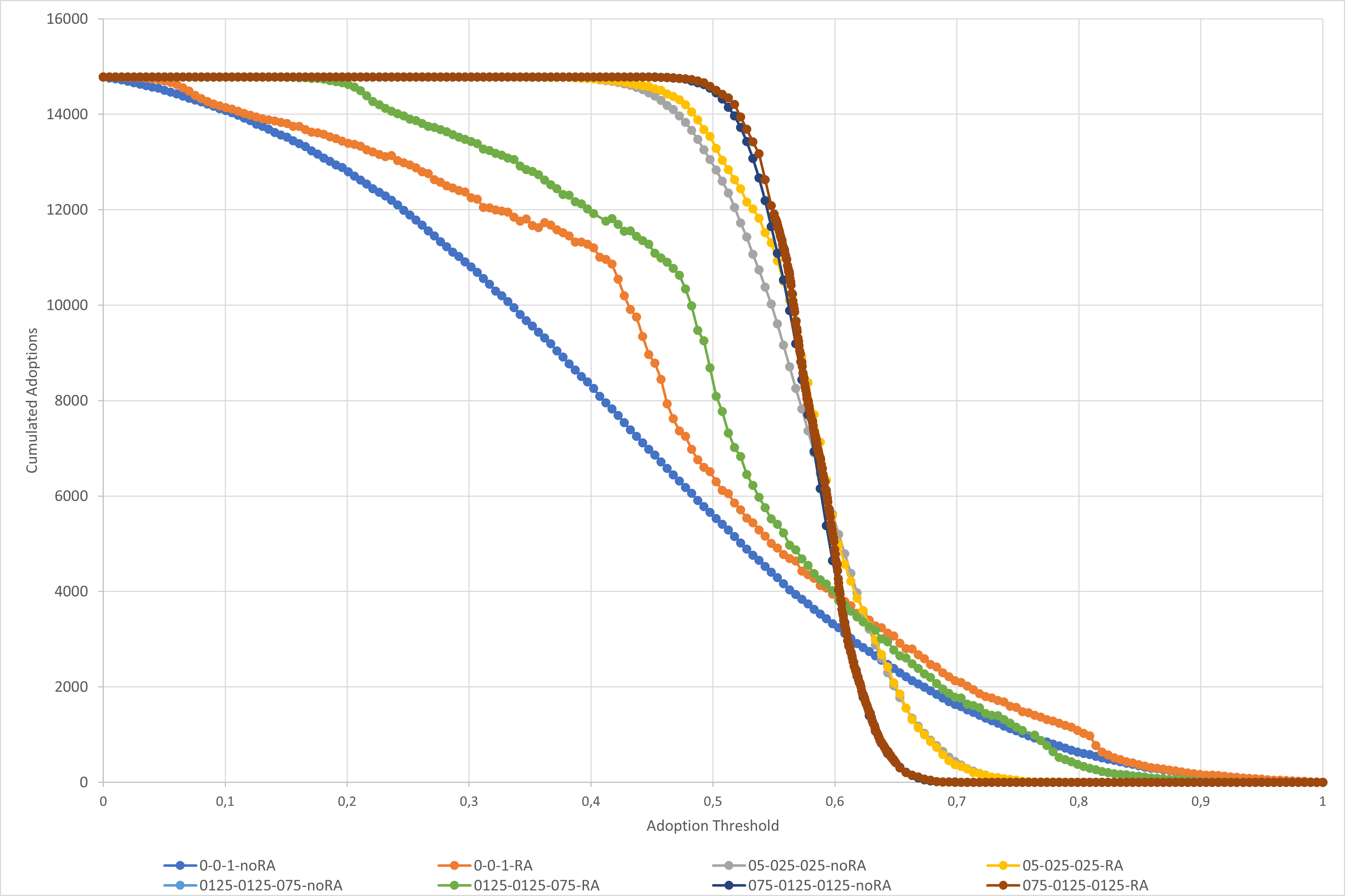
The remaining (sub-)scenarios on agents’ attitudes without allowing for opinion dynamics investigate the interaction of attitudes and the financial evaluation based on the systems’ NPV. These scenarios (II-05-025-025, II-025-05-025, II-025-025-05, II-0125-0125-075, II-0125-075-0125, II-075-0125-0125, II-033-033-033) show a monotonous decrease in adoptions that is smoother than the case of purely monetary evaluation (scenario II-1-0-0). For this case, a higher influence of monetary evaluation seems to imply a stronger decline in the cumulated adoption over time (as can be seen by the sharp decrease of adoption for scenarios II-075-0125-0125 and II-05-025-025 and the more gradual adoption decline curves of the scenarios where monetary evaluation plays a smaller role). However, in contrast to II-1-0-0 (where monetary evaluation is the sole decision factor), agent attitudes seem to be a moderating factor that smoothes out the decline of the adoption of the agents.

Scenario III

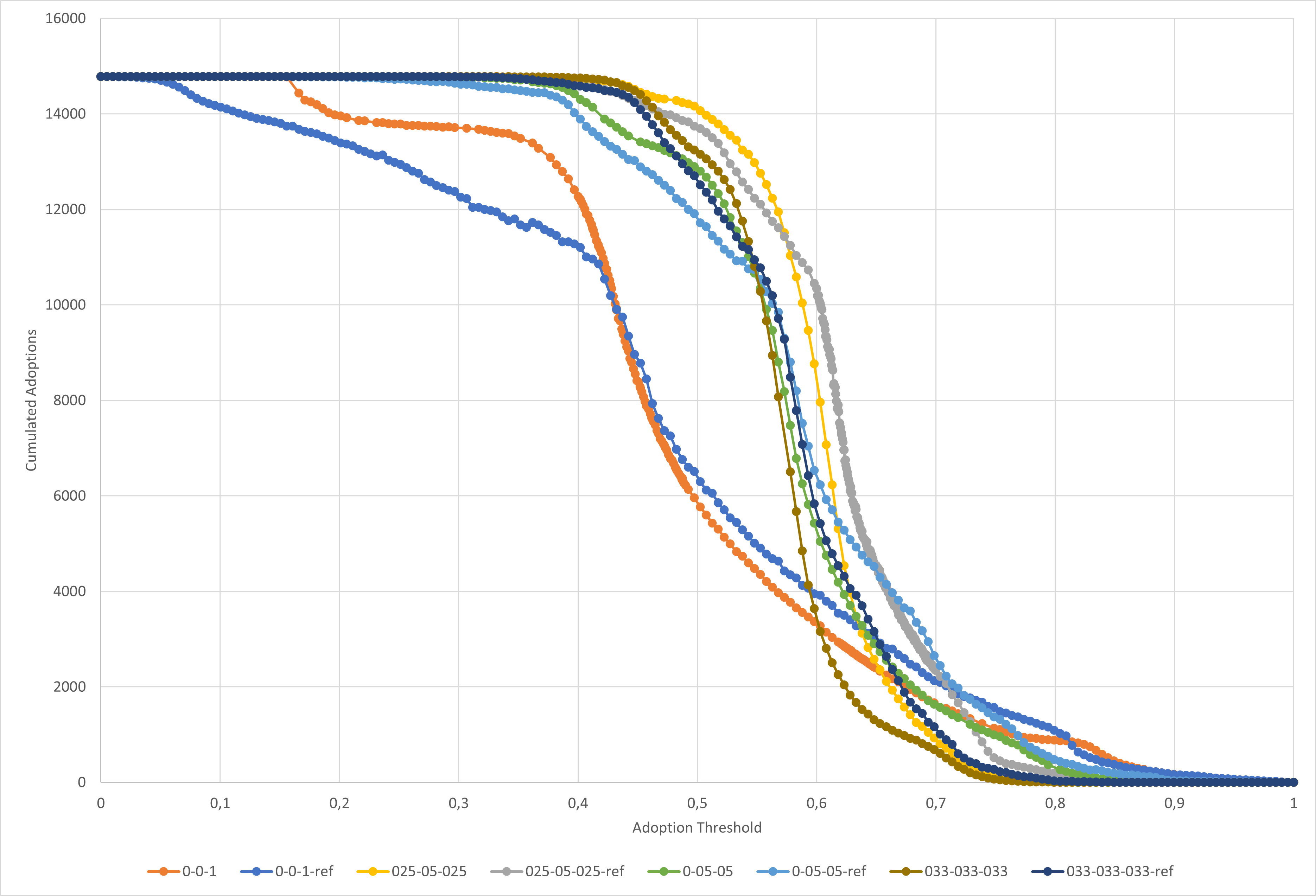
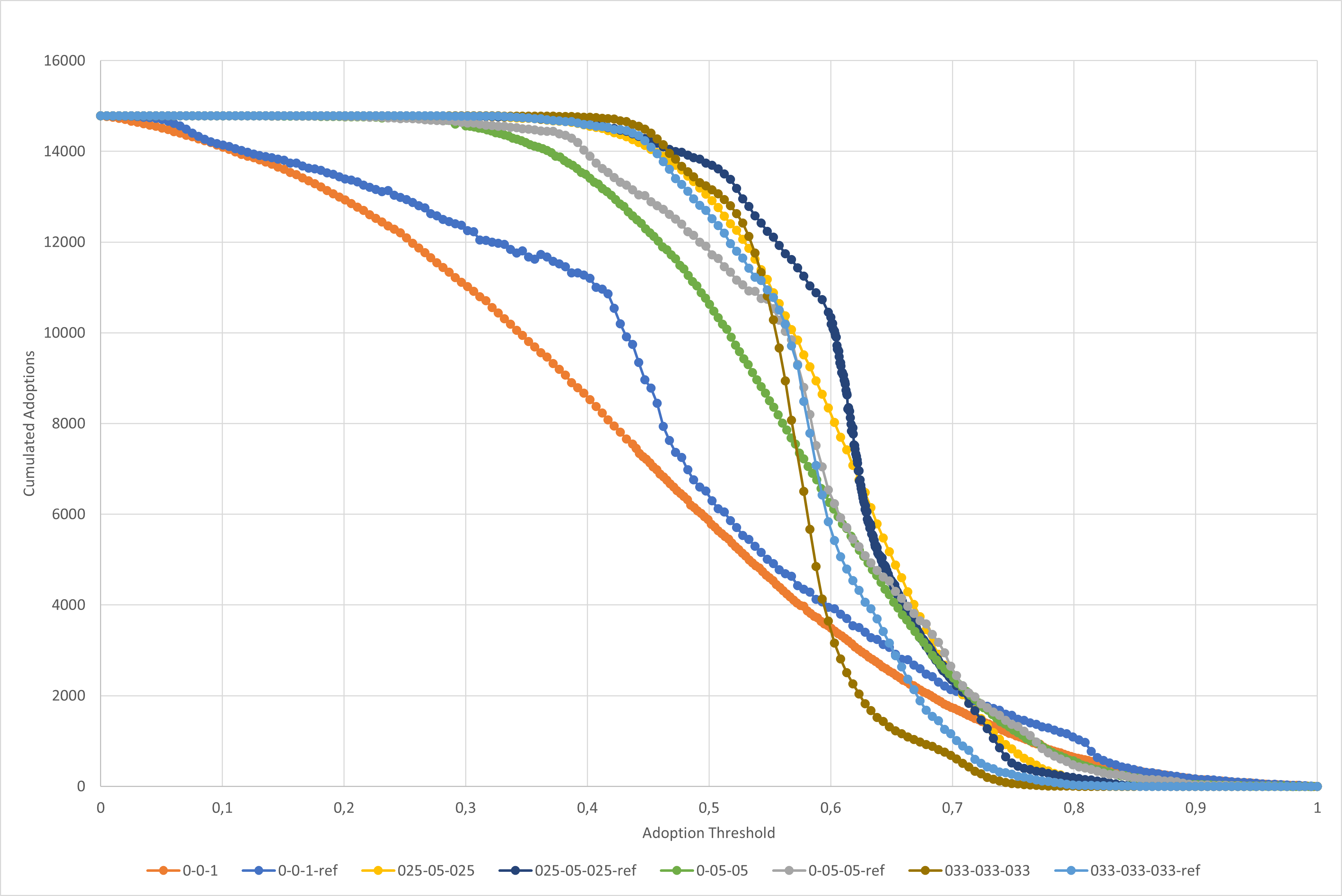
In order to analyze the influence of opinion dynamics on the adoption patterns, cumulated adoptions were investigated for scenarios that varied the influence of financial evaluation and the attitudes innovativeness and environmental awareness under influence of opinion dynamics through the relative agreement algorithm.

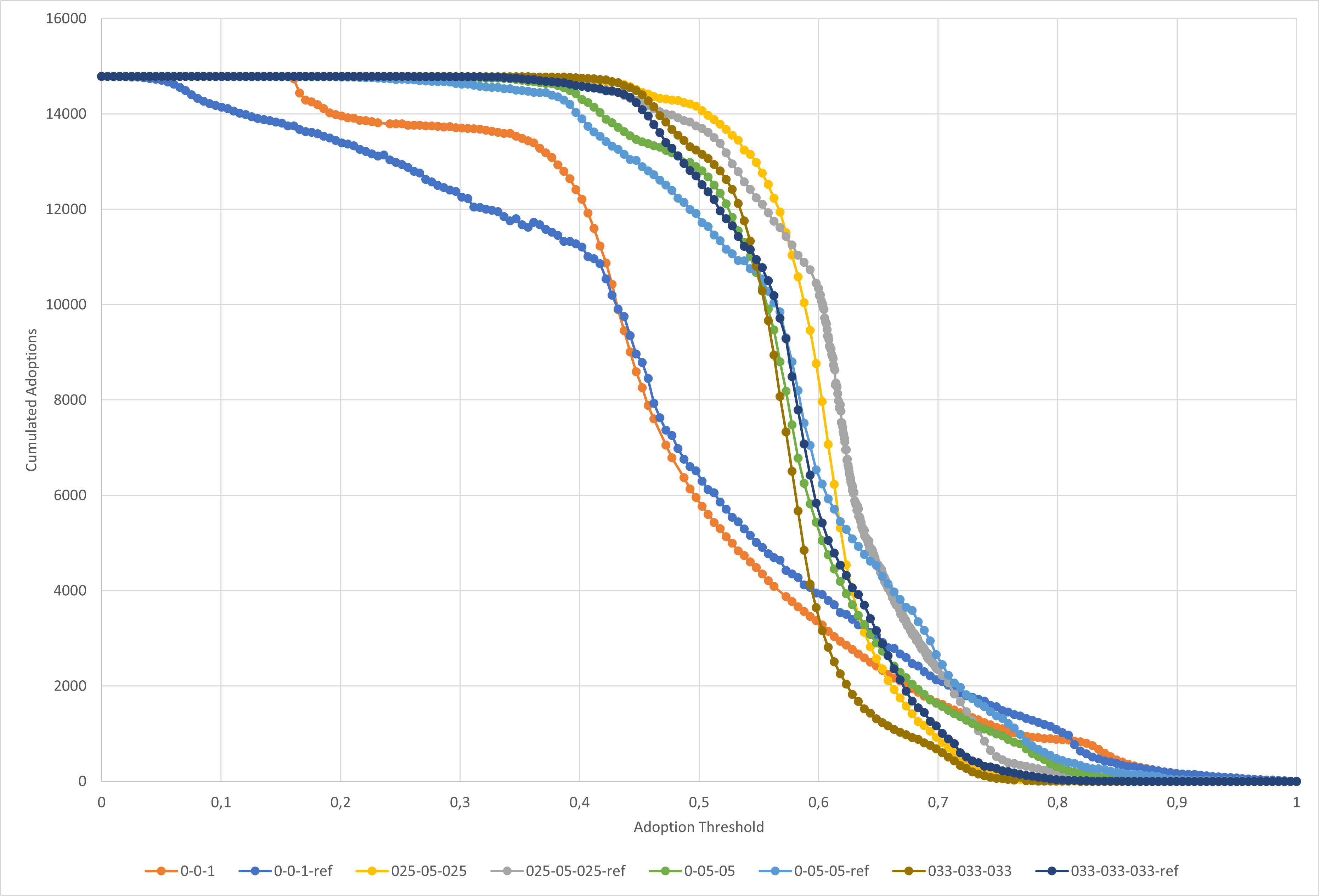
Overall, the adoption patterns as shown in Figure 17 are similar to the behavior seen in the scenarios without opinion dynamics (see Section 3.12, with less smooth transitions between cases. Figures 18 – 20 show scenarios with identical weights in a direct comparison where opinion dynamics were used and scenarios where this was not the case.

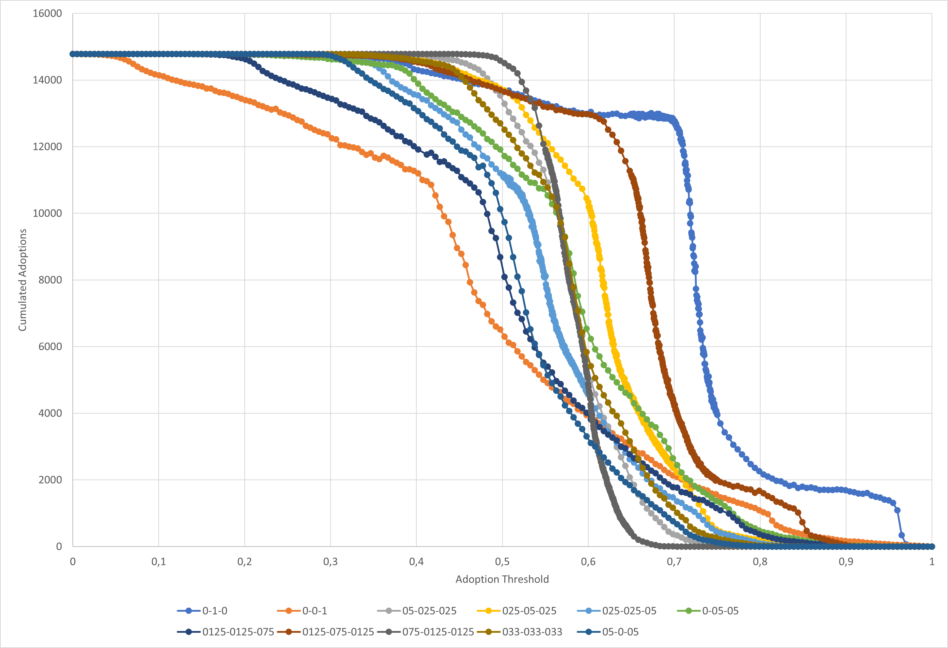
In order to explore the strength of opinion dynamics on the adoption patterns, parameter variations of the relative agreement algorithm were simulated for selected parameter combinations. The results of these simulations are shown in Figures 17 - 20.

The scenarios show near identical adoption behavior for small and large adoption threshold values for all cases except the scenario where the environmental attitude is the only determinant.

For the ‘middle region’ of the adoption threshold, where big quantitative simulation result differences are seen for comparatively small changes in the adoption threshold parameter (i.e. where the system reacts to the parameter in a more sensitive way), the parameter behavior is smoother for the case without opinion dynamics. In general, the same level of adoption is seen still with a higher adoption threshold for the case where opinion dynamics occur, indicating that they incentivize further spread of adoption as they lead to diffusion of more favorable attitudes towards the system. The degree to which this is the case differs, though.

Overall, three types of these behavior can be seen; In the case where the adoption depends solely on innovativeness (scenarios 0-0-1), the higher adoption with opinion dynamics is very clear. For cases where the decision influences are rather balanced (scenarios 025-025-05, 025-05-025, 0-05-05, 05-0-05, 033-033-033), a clear ‘bump’ is seen, where the adoption levels are shifted to a higher adoption threshold for a comparatively small region of the adoption threshold parameter (sub-)space. For the scenarios 075-0125-0125 and 05-025-025 barely any difference is seen in the adoption behavior between the cases with and without opinion dynamics.

The scenarios 0125-0125-075, 0-1-0 and 0125-075-0125 show somewhat different adoption behavior is seen. For the case where adoption is decided entirely by the environmental behavior (which also increases linearly throughout the simulation), a much slower decline in adoption is seen up to an adoption threshold of 0.7 from which on cumulated adoptions strongly decline before reaching another somewhat stable plateau, after which they feature another sharp decline. The case without opinion dynamics shows a much more gradual behavior.

A somewhat opposite behavior can be seen for the scenario 0125-0125-075, where both adoption curves are rather gradual, but where the case of opinion dynamics features a much more gradual adoption curve and the case without opinion dynamics shows a very steep decline in adoption in the parameter middle region.

Unsurprisingly, the scenario 0125-075-0125 shows a combination of these behaviors. As in 0-1-0, the adoption decline starts in a much later time with less of a plateau. As in the scenarios 0125-0125-075, the decline is much steeper than the reference scenario and then stabilizes. However, the roles are reversed as in the scenarios 0-1-0, with opinion dynamics leading to higher adoption numbers for a wider parameter band and then to a sharp decline behind the level of the case where no opinion dynamics take place.

Opinion dynamics strength

In addition to the influence of the relative agreement algorithm on the adoption patterns across scenarios, its intensity and directionality was investigated. For this, a set of scenarios were simulated that change the parameters of the relative agreement algorithm in order to increase or decrease the dynamics.

For this, the following scenarios were built (see Section 2.17):

1. III-C increased convergence (attitude gap 0.9, probability convergence 0.75, probability neutral 0.25, speed of convergence 0.25)
2. III-O decreased opinion dynamics (attitude gap 0.03, probability convergence 0.1, probability neutral 0.8, speed of convergence 0.03)
3. III-D increased divergence (attitude gap 0.9, probability divergence 0.75, probability neutral 0.25, speed of convergence 0.25)
4. III-E extremists (same as usual but with 0.75 extremists)

For the case where the convergence of the relative agreement algorithm is increased, the model behavior doesn’t change significantly (see Figure 21). Overall, it can be seen that that the decline in adoption numbers starts at a later point, but falls off more steeply. For scenarios with higher adoption thresholds, adoption behavior appears to be generally slightly higher than in the reference case. This suggests that the system is more sensitive to threshold changes in the ‘middle’ region where large adoption differences can be seen with little variation of the required utility to adopt. Yet, changes in this parameter region seem smoother, suggesting that the system responds more gradual towards this.

In contrast to the case of increasing convergence (i.e., more common application of the standard relative agreement algorithm), the scenarios IIID-* increase the divergence parameter, i.e. the probability that the inverse relative agreement algorithm will be applied. The results as visualized in Figure 22 show the same behavior as seen above. Inspection of common data points for the adoption threshold between the scenarios IIIC-* suggest identical adoption behavior between both cases; a comparison of the estimated implied function describing the adoption behavior for the scenarios¹⁴ found that the estimated functions have perfect or near-perfect equivalence for the investigated scenarios, suggesting that these dynamics play no role for the adoption behavior of households in these model configurations.

Decreasing the convergence parameters (scenario family IIIO-*) overall shows smoother adoption behavior, albeit in a different way to IIIC-* and IIID-*. The behavior shown in Figure 23 shows very gradual and smooth adoption curves throughout the investigated parameter range, with small variations of the required utility for adoption leading to small differences in the number of adopters. With the exception of scenario 033-033-033 where all weights are (almost) equal, the adoption curves lie under the reference case (with the exception of very small or very large adoption thresholds). The scenario 033-033-033 shows steeper adoption behavior than in the reference case, concentrating adoption differences in the parameter ranges of an adoption parameter of 0.5 and 0.65, which sees high sensitivity for the parameter.

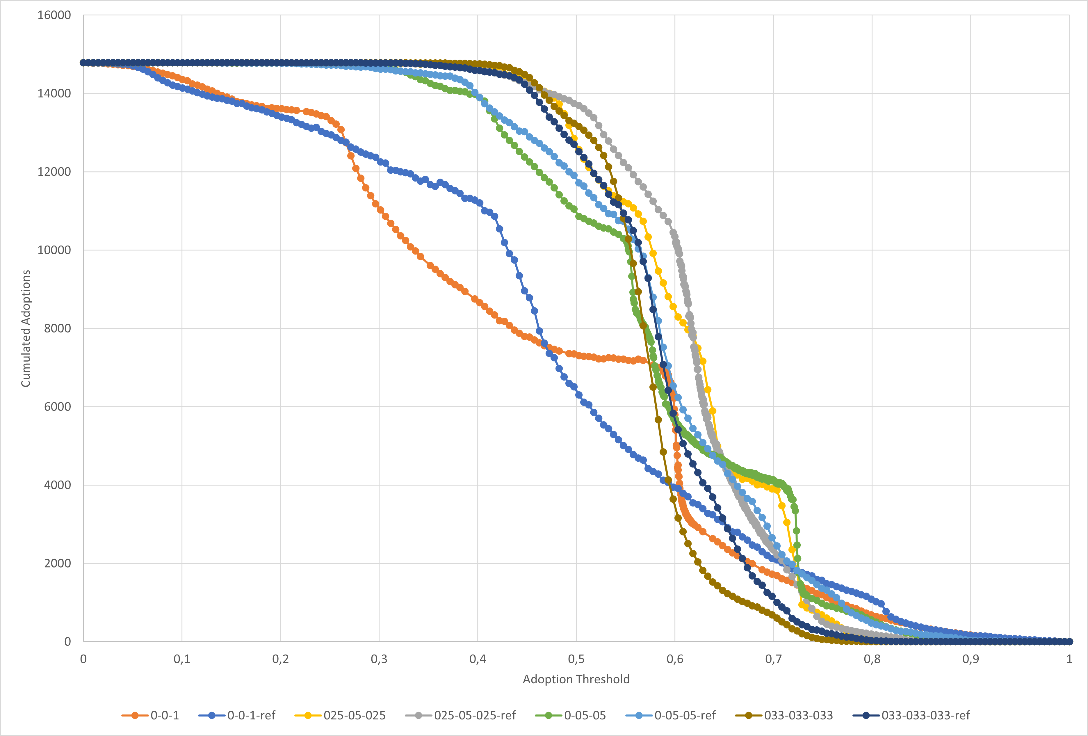
The last set of scenarios investigated with a focus on opinion dynamics (scenario family III-E) analyse the influence of extremists within the relative agreement algorithm. In all cases but where the decision factor weights are balanced (scenario IIIE-033-033-033), the adoption behavior shows to be more erratic than in the reference case. In these cases, the change in adoption patterns is rather gradual with increasing adoption threshold, while in certain parameter regions, adoption patterns differ strongly with minor changes in this threshold.

For scenario IIIE-0-0-1, adoption pattern changes become particularly sensitive around a threshold of 0.26 and 0.595, with the latter leading to very steep adoption drop pattern up to roughly 0.62. In the scenario IIIE-0-05-05, these drops occur at a higher threshold, with a minor drop around 0.4 and two steeper ones in the parameter region of 0.55 and 0.6 as well as 0.715 and 0.73, after which the adoption depression curve becomes flat again. Even stronger behavior is seen in the scenario IIIE-025-05-025 with two minor and two major drops in adoption behavior with increasing adoption threshold. The minor drops occur at 0.477 and 0.557, with the major one at 0.615 and 0.7. Overall, the patterns show certain tipping points where the system behavior changes qualitatively with minor changes in the adoption threshold. Increased extremism thus seems to support chaotic system behavior. The overall system behavior for the different scenarios with increased extremists can be seen in Figure 24.

Discussion

This section discusses the results of the exploratory analysis done in the Results Section and reflects on the taken approach. As exploratory modeling and theoretical exposition, the results primarily characterise the behaviour of the PVact model under the stated mechanisms and assumptions; they do not provide quantitative forecasts or validated effect sizes for the case study. Instead, they are used to illustrate the proposed modelling process and to motivate qualitative observations and discussion points for empirical and policy research on residential PV adoption and provide the basis for future work that is of more explanatory, or even predictive nature. Insights could also stimulate the debate or further research on measures to increase PV adoption.

Discussion of results

This article uses the agent-based model PVact to investigate how financial evaluation, normative pressure, and opinion dynamics affect household adoption dynamics under systematically varied scenario assumptions. This research sampled the parameter space across scenario groups by varying the weight of selected parameters to assess their influence on aggregate outcomes. While residential PV adoption is supported by a substantial empirical literature, the analysis in this article is exploratory rather than predictive: the results are interpreted as qualitative regime behaviour, sensitivities, and model-implied observations (e.g., tipping behaviour and relative mechanism leverage), not as quantitative effect-size estimates for the case study.

Scenario family I investigated model behavior under normative pressure and monetary evaluation. Focusing entirely on social or local pressure as determinants of the agents’ decision yielded systems that are dominated by chaotic behavior and that show very strong critical points. Combining both forms of normative pressure moderated this behavior somewhat. However, the system still exhibited the extreme behavior seen in the cases where this was studied in isolation. In contrast to this, the case of purely financial evaluation showed much more gradual behavior. This was especially the case from an aggregated perspective when the cumulative adoption throughout the entire simulation was viewed. After plateaus, the adoption curve showed roughly linear adoption degradation patterns. The dynamic analyses showed a concentration of simulated adoption in the first years of the simulation. This overall pattern shifted with higher requirements for the NPV needed for positive evaluation. Altogether, the monetary evaluation showed a more gradual distribution, acting as a moderating factor to the extreme behavior of normative pressure.

Finally, scenario family I combined the financial evaluation and normative pressure. In these scenarios, the strong characteristics of normative pressure dominated and the system showed extreme behavior. The analysis of the system behavior throughout different scenarios showed narrow parameter bands where adoption patterns varied from full adoption to no adoption whatsoever. In the most moderate case, normative pressure was lowest. Overall, bands in which strong behavior was shown are exceedingly narrow.

Scenario family II analysed the interplay of monetary evaluation and household attitudes without using opinion dynamics. The observed dynamics showed very gradual behavior throughout the variation of the adoption threshold in the static case where the cumulative adoption was analyzed. Attitude-based adoption further showed much smoother and more gradual behavior than the system behavior seen with monetary evaluation alone. Most scenarios exhibit behavior that is situated between the behavior seen where adoption depends fully either on environmentalist or innovative attitude, suggesting interpolation of the behavioral space by interpolation in the parameter space. The case of innovativeness presents a wide spread and a later drop of adoption numbers with increasing threshold than with environmental attitude. If the financial evaluation is considered alongside attitudinal factors, smoother behavior is seen than in the case of monetary evaluation alone. A stronger contribution of the monetary evaluation suggests a stronger decline in adoption behavior, with attitudes seeming to act as moderating factor for cumulative adoption behavior.

Scenario family III built on this analysis by including opinion dynamics based on the relative agreement algorithm in the simulation. The scenarios show similar macro-patterns and near identical behavior between scenarios both for small and large adoption threshold values, with the exception of the case where environmental attitude is the only determining factor. For more sensitive parameter regions, opinion dynamics seem to lead to less smooth behavior, with higher adoption in regions of higher adoption thresholds, implying that opinion dynamics incentivize the spread of adoption against higher resistance. Purely environmental attitude-driven behavior shows somewhat different behavior, exhibiting a combination of slow decline, adoption level plateaus and steep declines. Other scenario behavior is somewhat heterogeneous; some scenarios show prolonged adoption behavior for higher thresholds than the reference scenario (‘bumps’), some show slower adoption with plateaus, interrupted with steep decline, a third case shows more graduality where other scenarios show barely no influence of opinion dynamics.

Finally, Scenario family III also investigated the behavior when certain aspects of opinion dynamics are accentuated. It showed that increased convergence or divergence of the relative agreement algorithm generally had a rather minor influence, delaying the decrease in adoptions to a higher threshold and leading to more sensitivity in the parameter region where this occurred. Overall, this behavior was rather smooth, with slightly higher adoption numbers. A decrease in convergence showed smooth and gradual behavior with adoption curves generally lying under the reference case. The most extreme behavior was seen in the case where extremist behavior was accentuated. In this case, erratic behavior is seen in most scenarios, with regions that are very sensitive to changes in the adoption threshold and plateaus with little sensitivity. This suggests increased chaotic behavior and numerous tipping points with the introduction of a higher share of extremist agents.

It is important to note that these observations are valid for the studied model. While some aspects might very well translate to the studied system or could be generalized, the methodology does not allow for the transferability of these insights. For a more thorough discussion, see Edmonds et al. (2019). However, results suggest several qualitative observations that may inform empirical research and policy discourse. First, adoption dynamics are highly sensitive to normative pressure, with narrow threshold bands producing tipping-point behavior; this implies that interventions affecting perceived adoption prevalence and social visibility may generate discontinuous uptake changes rather than incremental effects. Second, monetary evaluation acts as a moderating mechanism: where adoption depends primarily on financial utility, uptake declines more gradually, and it can dampen—but not eliminate—tipping behavior induced by normative pressure. Third, opinion dynamics can shift adoption upward in regions of higher resistance (higher adoption thresholds), suggesting that diffusion of attitudes may be relevant to sustaining uptake when baseline willingness is limited. These observations show model behavior that may have real-world implications, but need further rigorous investigation to be taken as solid insights, as noted above.

Evaluation of the system approach

The article set out to address the following (slightly paraphrased) research questions:

• What is the relative influence of financial evaluation, normative pressure, agent attitudes and opinion dynamics, as well as their interactions, on the adoption behavior of rooftop PV in a municipal system on a system scale?
• How does the scenario-centered application of exploratory modeling to the parameter landscape investigated in this article inform the modeling process of rooftop photovoltaic adoption by household agents in a municipal energy system methodologically?

While the first question has been amply addressed in the Results Section and 2.6ff from a system perspective, the second evaluates the application of the developed methodology.

While there is a substantial empirical literature on residential PV adoption and its determinants, translating this evidence into municipal-scale parameterisation and validation remains challenging because reported effects are often context-dependent and interact with local heterogeneity and spatial constraints. In the discussed case study, the available evidence supports specifying plausible mechanisms and defensible parameter choices, but is insufficient to meet stricter requirements for predictive or strongly explanatory modelling (Edmonds et al. 2019). Therefore, model evaluation is focused on transparency, internal coherence, and sensitivity of qualitative behaviours rather than on forecast accuracy.

To better understand the system and analyze its system behavior under different parameterizations, the parameter landscape was evaluated to concrete scenario designs that surveyed the parameter landscape by varying decision parameters and their relative weights based on a free parameter (adoption threshold) based on the guidelines for exploratory modeling in Section 2.6.

Three scenario families focusing on different decision factors and their relative weights indicated rich model behavior, varying between very gradual and smooth behavior via scenarios exhibiting more sensitive parameter regions to erratic and chaotic behavior with extreme sensitivities. The approach was thus suited to study the macro behavior of the system in different scenarios. Within the scenarios, the approach showed parameter regions where the model yielded interesting behavior. This indicated adoption threshold intervals where a more in-depth investigation of model aspects would most likely yield interesting behavior. It also informed the choice of weights of decision determinants for future investigations.

Through this, it informed the modeling process. However, it did not yield the insight necessary to construct an explanatory or predictive model of the investigated system, nor did it address any of the calibration challenges noted in Johanning et al. (2022). As a theoretical exposition, the analysis gave insight into the model rather than the modeled system (Edmonds et al. 2019), strictly speaking not yielding comprehension beyond further theoretical exposition. However consistent this would be ontologically, our approach should be valuable to modelers of municipal energy systems, household decisions or diffusion of low-carbon technologies, as well as empirical researchers and political actors. To empirical researchers, the model can suggest hypotheses to test in the real world, whereas for political actors, the systems sensitivities might suggest sensitivities that could occur in the real world. Particularly the sensitivity of the model to normative pressure and opinion dynamics could inform discussions on the right political tools to promote change. This might be increasingly important given the rise of disinformation and authoritarianism observed in recent years. However, models are build on simplifications and abstractions and can solely serve as inspiration for action in the real world. The use for modelers of municipal energy systems, household decisions or diffusion of low-carbon technologies is manifold. The empirically and theoretically grounded model design presented in this article can inform modeling choices of modelers, whereas the simulation results identify behavior of model components that might occur in a similar fashion in their models, potentially contributing to explain the model behavior. The methodology presented in this article might be valuable for modelers that want to get a deeper insight into how their model unfolds and is intended to enrich the discourse on modeling approaches.

Analogously to Rai & Robinson (2015), we use an empirically well-grounded ABM to explore different system designs under behavioral and social uncertainty. In their words, this provided a “virtual laboratory” where different policy options could be explored. This is in line with the approach of Kwakkel (2017), Bankes (1993), Bankes et al. (2002), Bankes et al. (2013) which allows for the exploration of different adoption pathways under deep uncertainty in contrast to exact precision tools. A key contribution of the model is to reveal how different uptake patterns emerge from different system configurations, allowing for an exploration of the parameter space. As noted in (Moallemi et al. 2020) we thus use the exploratory approach as thinking aid that allows to explore implications of (alternative) assumption systematically in problems with deep uncertainty in an outcome space.

Limitations

The article discussed the system behavior of the PVact model on the basis of different decision determinants and system assumptions. While the system indicated a range of interesting dynamics as it is, this research was done within a given set of constraints that are discussed in the following. The discussion of the limitations is structured by limitations of the model, the employed scenarios and the chosen approach.

The investigated model has several limitations. While for normative pressure and attitudes, the drivers of adoption were operationalised similarly to existing work, the financial evaluation was rather unconventional. Alternative formulations of the monetary evaluation could have been explored, and the model structure could have been investigated more thoroughly. However, based on the chosen research design, the weights of the decision factors within the model formulation were seen to be more important at this point and it was decided not to dilute the focus of this work for this. As with different approaches to financial evaluation, alternative model structures could have been investigated. The process model was based on the theory of innovation diffusion (Rogers 2003) and focus groups interviews analyzed throughout model development (Scheller et al. 2021). Additionally, the model included different simplifications, such as not differentiating between owners and renters or not considering restrictions such as heritage issues or tree shadowing (as brought up during the focus groups). Similarly, logistical issues (such as installation capacities, financing etc.) were not included in the model. These modeling decisions were taken to reduce (already high) model complexity and for these factors we found relatively little empirical evidence (in focus group research) and accessible data.

While DOI gave more theoretical grounding to the model and the focus groups increased the empirical grounding, other model structure elements were just as possible. Different model structures would likely result in different results, although similar model dynamics might have been seen overall. Finally, many actors play a role in a dynamic network of stakeholders (Scheller et al. 2021). While their inclusion was thoroughly considered in the development of the model, complexity reduction was prioritized and the introduction of new actors scheduled for a later point.

While the model underwent extensively theoretical, data and internal validation, serious issues were encountered during operational validation (Johanning et al. 2022). By investigating the model behavior through a range of scenarios and the core parameter adoption threshold, an important part of the calibration process was done. However, other free parameters, such as the interest points and interest threshold were not part of the calibration. While stochasticity was the main reason that calibration was difficult (Johanning et al. 2022), it was deemed essential to the model from a phenomenological perspective. Stochasticity could also have been addressed by a focus on the intention-behavior-gap. While the empirical data explains almost 40% of the adoption intention, a significant part of the (non-)adoption behavior could not be addressed in the model. This was complemented with the empirical (survey-based) data stemming from only one survey. Through this, data that is most likely dynamic was parameterized as static.

The most obvious limitation with the scenario approach was the limited number of investigated scenarios. The model was theoretically based primarily on the theory of innovation diffusion and theory of planned behavior. Other choices would have resulted in different determinants that could have been investigated and some determinants of household decisions (such as normative motives, beliefs, norms or behavioral control) were not studied. The chosen decision factors were carefully based on research; however, other factors could have been overlooked or might not have been ruled out with a different research approach. The investigated scenario families further left out the interest threshold. Immediate adoption of technologies is highly unrealistic, which is why PVact includes interest dynamics. The model exploration, however, focused on the adoption threshold and kept the gathered interest points and the interest threshold constant within the scenarios. Due to the focus on the overall (cumulative) adoption, this limitation should only have a minor influence on the results for the scenario families II and III. Still, these dynamics might have been relevant and should be part of future investigations. Finally, the investigation focused on case-study specific pararameters from the city of Leipzig (Germany) and the empirical survey. Due to the specificity of the case-study data and its static nature, results may not be generalizable both to other local contexts and other model designs. This would require careful experiments and discussions on similarities and differences between model results.

In addition to the limitations coming with the model and scenarios, the approach had its own limitations. This research brought together the modeling classes of exploratory modeling and theoretical exposition. The article is thus in danger of suffering from the limitations of both classes, particularly the lack of connection between simulations to the observed world and results for theoretical expositions, preventing conclusions about the modeled system based on the model. While exploratory modeling showed to be a profitable approach for a model of the investigated complexity, this approach gives comparatively little insight in the inner workings of the model and does not add explanatory or predictive adequacy and shouldn’t be understood as quantitative forecasts for PV diffusion. While a focus on specific model aspects could have given deeper insight in these model aspects, it would have taken resources from the exploration of the ensemble landscape.

Conclusion

Discussion summary

Analysing the different system dynamics found a range of system behaviors for different parameterizations formalized in three scenario families. The most dominant dynamics were seen with normative pressure and opinion dynamics with increased fraction of extremists. Of these, normative pressure exhibited the most extreme behavior, with chaotic dynamics, strong critical points and very narrow parameter bands in which it was sensitive to the model parameters, and was barely moderated by interlacing it with monetary evaluation.

In contrast to this, both monetary evaluation and attitude-based decision making showed rather smooth and gradual behavior. Scenarios basing the decision on attitude without using opinion dynamics generally interpolated the behavior seen in the extreme cases where the adoption decision depended on only one variable.

Opinion dynamics suggest to lead to more sensitivity in the middle parameter region. They suggest to have a stabilizing influence for adoption threshold parameter regions where the required utility to adopt is either high or low. For the middle region, opinion dynamics seem to increase parameter sensitivity and seem to have a role in tipping the system. However, they also seem to lead to higher adoption in regions of higher threshold, suggesting a role in overcoming agent resistance.

The most extreme behavior for opinion dynamics was seen with the case where extremism was raised in the population. These systems show much more erratic behavior with regions of varying sensitivity, suggesting chaotic behavior and tipping points. While this was not as strong as in the case of normative pressure, it showed strong dynamics, especially if contrasted to the more ‘moderate’ cases discussed above.

The methodological discussion in Section 4.9 showed that the chosen methodology could indicate qualitatively distinct macro-behavior in some scenario families and concluded that the exploratory modeling methodology informed an understanding of the modeling process. It proved valuable in surveying the model landscape and applicable to a modeling context where not enough knowledge existed to make robust predictions or prove the value of an explanation within reasonable doubt. Conservatively speaking, as theoretical exposition, it should only inform the narrow scope of the studied model. However, the discussion argued that, while no direct insight into the modeled phenomenon could be given, it suggested various aspects that would advance the understanding of the studied system and the system overall. This is further discussed below in Section 5.9ff.

Contribution

This research contributed to the discourse in different ways. Based on the seminal work by Bankes (1993) it developed, applied and analyzed a wide range of decision factors for household decisions in the context of the ABM diffusion model PVact on the basis of three scenario families. While much of the contribution of this article is specific to the model, the developed approach is very likely to transfer to other models.

Methodologically, this article built on the exploratory paradigm of Bankes (1993) and applied the more abstract notions to a concrete research design. Within the research design, a number of scenario families were designed based on the theoretical basis of the PVact model. A methodology for systematic sampling and surveying the parameter landscape was developed, with the scenarios building on one another without redundancy. It is imperative to bear in mind that this methodology was not focused on predictive modeling and the model is not suited to make forecasts on the actual development of rooftop PV in the studied municipality, but is firmly rooted in exploratory modeling, showing the model behavior with variation of the importance of the model (decision) parameters.

This methodology is ready to be adapted to other modeling contexts. This article thus provides a transferable research design that can inform other application contexts and future work.

Future work

While this article gave a comprehensive overview of the model behavior under a range of decision factors, Section 4.10 indicated much potential for building on this research. Future work can be coarsely classified in extending the model and refining the approach.

The model could be extended theoretically by adopting further behavioral or context-specific theories and decision factors that have been left out in this research or a more intensive investigation of the financial evaluation. Empirically, the model could be extended by a further survey that would allow for a more dynamic perspective on the variables that were parameterized with the static snapshot of the included survey.

Beyond this future work to strengthen the grounding of the model, it could be extended by including more actors (Scheller et al. 2021) or complementory technologies such a storages or alternative generation sources. Finally, the model is probabilistic in nature, making calibration of the model difficult. While different solutions to this were developed (Johanning et al. 2022), this warrants more research. Future work could focus on this to put the model on a more stable basis.

Furthermore, the limited generalizability of the model could be extended by applying the model and methodology to different local contexts or by investigating the robustness of the results to modifications of the model. Studying which characteristics of other local contexts change model results in what way could give indicators on the influence of the local context characteristics and more fundamental and generalizable model dynamics and spatio-economic-social aspects. By modifying the model, robust model characterics could be identified that generalize across model idiosyncracies.

In addition to building on the model, the approach taken in this paper could be extended. Future work could go beyond conventional scenario discovery, e.g. by considering dynamics and the techniques in Steinmann et al. (2020), most of all clustering of internally similar time-series data. As a study on policy analysis, it could focus on designing and exploring adaptive policies, complementing the exploratory modeling approach.

From the perspective of the investigative focus, a research design with a bigger focus on explanation than exploration could be chosen. This could feed into the discussion on the role of individual decision factors or decision process steps, requiring a more focused and deeper perspective on singular model elements. Finally, future work could go beyond scalar parameters through focusing more on random distributions and analyze multi-dimensional model variables. Going beyond scalar parameters would be viable future work, particularly when more model contingencies are explored, e.g., through methods such as inverse generative social sciences (Epstein et al. 2023). This would also open up further avenues in model calibration, e.g., through calibrating on multiple milieus or milieu groups and by calibrating on the moments of the distributions based on historic data, as has been discussed in [redacted for blind review].

Additionally, Bankes et al. (2013) mentions a number of algorithms that support exploratory modeling and analysis that could be applied and extended in order to deepen the exploratory work done in this article.

References

ABITZ, D., Johanning, S., Vogt, E., Scheller, F., & Bruckner, T. (2024). ODD+D protocol of the agent-based rooftop photovoltaic diffusion model PVact. Available at: https://zenodo.org/records/12818346

ALIPOUR, M., Salim, H., Stewart, R. A., & Sahin, O. (2021). Residential solar photovoltaic adoption behaviour: End-to-end review of theories, methods and approaches. Renewable Energy, 170, 471–486. [doi:10.1016/j.renene.2021.01.128]

AL Irsyad, M. I., Halog, A., & Nepal, R. (2019). Estimating the impacts of financing support policies towards photovoltaic market in Indonesia: A social-energy-economy-environment model simulation. Journal of Environmental Management, 230, 464–473. [doi:10.1016/j.jenvman.2018.09.069]

BANKES, S. (1993). Exploratory modeling for policy analysis. Operations Research, 41(3), 435–449. [doi:10.1287/opre.41.3.435]

BANKES, S., Lempert, R., & Popper, S. (2002). Making computational social science effective. Social Science Computer Review, 20(4), 377–388. [doi:10.1177/089443902237317]

BANKES, S., Walker, W., & Kwakkel, J. (2013). Exploratory modeling and analysis. In S. I. Gass & M. C. Fu (Eds.), Encyclopedia of Operations Research and Management Science. Berlin Heidelberg: Springer. [doi:10.1007/978-1-4419-1153-7_314]

BAUSKE, E., Kibbe, A., & Kaiser, F. G. (2022). Opinion polls as measures of commitment to goals: Environmental attitude in Germany from 1996 to 2018. Journal of Environmental Psychology, 81, 101805. [doi:10.1016/j.jenvp.2022.101805]

BRATMAN, M. E. (1999). Intention, Plans, and Practical Reason. Stanford, CA: CSLI Publications.

DANIELIS, R., Scorrano, M., Massi Pavan, A., & Blasuttigh, N. (2023). Simulating the diffusion of residential rooftop photovoltaic, battery storage systems and electric cars in Italy. An exploratory study combining a discrete choice and agent-based modelling approach. Energies, 16. [doi:10.3390/en16010557]

DEFFUANT, G., Amblard, F., Weisbuch, G., & Faure, T. (2002). How can extremism prevail? A study based on the relative agreement interaction model. Journal of Artificial Societies and Social Simulation, 5(4), 1.

DERMONT, C., Ingold, K., Kammermann, L., & Stadelmann-Steffen, I. (2017). Bringing the policy making perspective in: A political science approach to social acceptance. Energy Policy, 108, 359–368. [doi:10.1016/j.enpol.2017.05.062]

EDMONDS, B., Le Page, C., Bithell, M., Chattoe-Brown, E., Grimm, V., Meyer, R., Montañola-Sales, C., Ormerod, P., Root, H., & Squazzoni, F. (2019). Different modelling purposes. Journal of Artificial Societies and Social Simulation, 22(3), 6. [doi:10.18564/jasss.3993]

EPSTEIN, J. M., Garibay, I., Hatna, E., Koehler, M., & Rand, W. (2023). Special section on "Inverse Generative Social Science": Guest editors’ statement. Journal of Artificial Societies and Social Simulation, 26(2), 10. [doi:10.18564/jasss.5085]

EUROSTAT. (2024). Eurostat: Energy consumption in households. Available at: https://ec.europa.eu/eurostat/statistics-explained/index.php?title=Energy_consumption_in_households

GRANT, C. A., & Hicks, A. L. (2020). Global warming impacts of residential electricity consumption: Agent-based modeling of rooftop solar panel adoption in Los Angeles County, California. Integrated Environmental Assessment and Management, 16(6), 1008–1018. [doi:10.1002/ieam.4315]

IEA. (2021). Net zero by 2050. Available at: https://www.iea.org/reports/net-zero-by-2050

JOHANNING, S., Abitz, D., Scheller, F., & Bruckner, T. (2023). The influence of financial benefits and peer effects on the adoption of residential rooftop photovoltaic systems. 2023 19th International Conference on the European Energy Market (EEM). [doi:10.1109/eem58374.2023.10161765]

JOHANNING, S., Abitz, D., Schulte, E., Scheller, F., & Bruckner, T. (2022). PVactVal: A validation approach for agent-based modeling of residential photovoltaic adoption. 18th International Conference on the European Energy Market (EEM), Ljubljana, Slovenia. [doi:10.1109/eem54602.2022.9921039]

JOHANNING, S., Scheller, F., Abitz, D., Wehner, C., & Bruckner, T. (2020). A modular multi-agent framework for innovation diffusion in changing business environments: Conceptualization, formalization and implementation. Complex Adapt Syst Model, 8(8). [doi:10.1186/s40294-020-00074-6]

KAHNEMAN, D., & Tversky, A. (1979). Prospect theory: An analysis of decision under risk. Econometrica, 47(2), 263. [doi:10.2307/1914185]

KAKOULAKI, G., Taylor, N., Szabo, S., Kenny, R., Chatzipanagi, A., & Jäger-Waldau, A. (2024). Communication on the potential of applied PV in the European Union: Rooftops, reservoirs, roads (R³). EPJ Photovoltaics, 15, 2. [doi:10.1051/epjpv/2023035]

KWAKKEL, J. H. (2017). The exploratory modeling workbench: An open source toolkit for exploratory modeling, scenario discovery, and (multi-objective) robust decision making. Environmental Modelling and Software, 96, 239–250. [doi:10.1016/j.envsoft.2017.06.054]

MACAL, C. M., Graziano, D. J., & Ozik, J. (2014). Modeling solar pv adoption: A social-behavioral agent-based framework. AAAI Technical Report FS-14-02.

MOALLEMI, E. A., Kwakkel, J., de Haan, F. J., & Bryan, B. A. (2020). Exploratory modeling for analyzing coupled human-natural systems under uncertainty. Global Environmental Change, 65, 102186. [doi:10.1016/j.gloenvcha.2020.102186]

MOGLIA, M., Nygaard, C. A., Glackin, S., Cook, S., & Tapsuwan, S. (2022). Hybrid approach for modelling the uptake of residential solar PV systems, with case study application in Melbourne, Australia. Journal of Artificial Societies and Social Simulation, 25(4). [doi:10.18564/jasss.4921]

NORLING, E. (2004). Folk psychology for human modelling: Extending the BDI paradigm. Proceedings of the Third International Joint Conference on Autonomous Agents and Multiagent Systems, 2004. AAMAS 2004. [doi:10.65109/pymb3281]

NURWIDIANA, N., Sopha, B. M., & Widyaparaga, A. (2022). Simulating socio-technical transitions of photovoltaics using empirically based hybrid simulation-optimization approach. Sustainability (Switzerland), 14(9). [doi:10.3390/su14095411]

PALMER, J., Sorda, G., & Madlener, R. (2015). Modeling the diffusion of residential photovoltaic systems in Italy: An agent-based simulation. Technological Forecasting and Social Change, 99, 106–131. [doi:10.1016/j.techfore.2015.06.011]

RAI, V., & Robinson, S. A. (2015). Agent-based modeling of energy technology adoption: Empirical integration of social, behavioral, economic, and environmental factors. Environmental Modelling and Software, 70, 163–177. [doi:10.1016/j.envsoft.2015.04.014]

ROGERS, E. M. (2003). Diffusion of Innovations. New York, NY: Free Press.

SCHELLER, F., Doser, I., Schulte, E., Johanning, S., McKenna, R., & Bruckner, T. (2021). Stakeholder dynamics in residential solar energy adoption: Finding from focus group discussions in Germany. Energy Research and Social Science, 76(5). [doi:10.1016/j.erss.2021.102065]

SCHELLER, F., Schulte, E., Johanning, S., Geyler, S., Moritz, M., & Bruckner, T. (2022). Beschreibung der realen fallstudien als forschungsobjekt für die modellbezogenen analysen. In Agentenbasierte Modellierung urbaner Transformationsprozesse (pp. 21–38). Berlin: Logos Verlag. [doi:10.30819/5413.02]

SCHIERA, D. S., Minuto, F. D., Bottaccioli, L., Borchiellini, R., & Lanzini, A. (2019). Analysis of rooftop photovoltaics diffusion in energy community buildings by a novel GIS- and agent-based modeling co-simulation platform. IEEE Access, 7, 93404–93432. [doi:10.1109/access.2019.2927446]

SCHUENEMANN, C., Johanning, S., Herold, H., & Bruckner, T. (2024). Modelling the behaviour in socio-technical systems for policy assessment - A comparison of modelling approaches using the example of Sponge City concept implementation. Journal of Cleaner Production, 462, 142722.

SCHUENEMANN, C., Johanning, S., Reger, E., Herold, H., & Bruckner, T. (2024). Complex system policy modelling approaches for policy advice - Comparing systems thinking, system dynamics and agent-based modelling. Political Research Exchange, 6(1).

SCHULTE, E., & Scheller, F. (2022). In Empirische Verankerung der Haushaltsagenten und ihres Photovoltaik-Investitionsverhaltens (pp. 129–138). Berlin: Logos Verlag. [doi:10.30819/5413.10]

SCHULTE, E., Scheller, F., & Johanning, S. (2022). Modellierung von haushaltsseitigen entscheidungsprozessen zur adoption von aufdach-photovoltaik: Theorie und umsetzung. In Agentenbasierte Modellierung urbaner Transformationsprozesse. Smart Utilities And Sustainable Infrastructure Change. Studien zu Infrastruktur und Ressourcenmanagement, Bd. 12 (pp. 39–50). Berlin: Logos Verlag. [doi:10.30819/5413.03]

SIMÕES, F. (2016). Consumer behavior and sustainable development in China: The role of behavioral sciences in environmental policymaking. Sustainability, 8(9), 897.

STEINMANN, P., Auping, W. L., & Kwakkel, J. H. (2020). Behavior-based scenario discovery using time series clustering. Technological Forecasting and Social Change, 156. [doi:10.1016/j.techfore.2020.120052]

SUNDARAM, A., Gonçalves, J., Ghorbani, A., & Verma, T. (2024). Network dynamics of solar PV adoption: Reconsidering flat tax-credits and influencer seeding for inclusive renewable energy access in Albany county, New York. Energy Research and Social Science, 112. [doi:10.1016/j.erss.2024.103518]

VAN DER KAM, M, Lagomarsino, M., Azar, E., Hahnel, U. J. J., & Parra, D. (2024). An empirical agent-based model of consumer co-adoption of low-carbon technologies to inform energy policy. Cell Reports Sustainability, 1, 12. [doi:10.1016/j.crsus.2024.100268]

VIBRANS, L., Schulte, E., Morrissey, K., Bruckner, T., & Scheller, F. (2023). Same same, but different: Explaining heterogeneity among potential photovoltaic adopters in Germany using milieu segmentation. Energy Research and Social Science, 103, 103212. [doi:10.1016/j.erss.2023.103212]

VLAEV, I. (2018). Local choices: Rationality and the contextuality of decision-making. Brain Sciences, 8(1), 8. [doi:10.3390/brainsci8010008]

WANG, G., Zhang, Q., Li, Y., & Li, H. (2018). Policy simulation for promoting residential PV considering anecdotal information exchanges based on social network modelling. Applied Energy, 223, 1–10. [doi:10.1016/j.apenergy.2018.04.028]

ZHANG, H., Vorobeychik, Y., Letchford, J., & Lakkaraju, K. (2014). Predicting rooftop solar adoption using agent-based modeling. [doi:10.1007/s10458-016-9326-8]

ZHANG, N., Lu, Y., Chen, J., & Hwang, B. G. (2022). An agent-based diffusion model for residential photovoltaic deployment in Singapore: Perspective of consumers’ behaviour. Journal of Cleaner Production, 367. [doi:10.1016/j.jclepro.2022.132793]