Heterogeneity in Agent-Based Models

,
,
and
aUniversity of Leeds, Leeds, United Kingdom; bKings College London, London, United Kingdom.
Journal of Artificial
Societies and Social Simulation 29 (2) 5
<https://www.jasss.org/29/2/5.html>
DOI: 10.18564/jasss.5872
Received: 25-Feb-2025 Accepted: 23-Feb-2026 Published: 31-Mar-2026
Abstract
Agent-based models are flexible tools that allow modellers to capture heterogeneity in agent attributes, characteristics, and behaviours. In this paper, heterogeneity is defined as agent granularity, referring to the level of detail used to describe agent attributes, behaviours, interaction processes, and decision-making rules. However, the increased complexity associated with greater levels of heterogeneity, and hence more parameters, can make the already challenging process of model calibration even more difficult. While modellers recognise the importance of calibration, the issue of uniquely determining model input based on a given output, known as parameter identification, is often overlooked. A central point of this study is that identifiability crucially depends on the outcomes or summary statistics chosen for calibration: even a well-specified model may become empirically uninformative if the selected statistics are not sufficiently sensitive to parameter variation. This paper argues that one significant impact of increasing heterogeneity in an agent-based model is the parameter identification problem, where the effects of model inputs cannot be uniquely distinguished in model outputs. To address this issue, the paper presents a comparative study of homogeneous and heterogeneous scenarios in agent-based models. Using a simple contagion case study model and approximate Bayesian computation for calibration, the study demonstrates that introducing heterogeneity reduces the accuracy of parameter calibration compared to the homogeneous case. This decline in accuracy is attributed to the difficulty in isolating the effects of the additional parameters introduced by heterogeneity. Rather than proposing computational fixes, the paper situates these findings within the broader methodological debate between KISS (“Keep It Simple, Stupid”) and KIDS (“Keep It Descriptive, Stupid”) strategies, highlighting how the trade-off between descriptive realism and tractability directly shapes the reliability of inference from ABMs.whose insight, collaboration, and scholarship greatly
contributed to this work and to the field.
Introduction
Agent-based models (ABMs) are well-known for their use in analysing various systems’ inherent and intricate complexities (Buchmann et al. 2016). They can uncover system patterns and characteristics of large-scale hierarchical structures from simple individual-level processes. Simulating a system with ABMs has its advantages, including the ability to capture heterogeneity (Bonabeau 2002). In this paper, heterogeneity is understood as agent granularity, encompassing variation in agent attributes, behavioural rules, and interaction processes.
Modelling a system heterogeneously often enriches the understanding and interpretability of the system’s dynamics; it connects attributes to observed behaviours and then to model outcomes. The insights gathered from connecting these facets can uncover valuable information about the target system that may have otherwise remained unknown. For example, in epidemiological modelling, connecting attributes to behaviours and outcomes can provide valuable insights into innovative policy approaches for containment (Bavel et al. 2020; Gulden et al. 2021; Reeves et al. 2022; Vermeulen et al. 2021).
This paper uses epidemic models as a case study to illustrate the impact of heterogeneity on simulating population differences and evaluating interventions (Berestycki et al. 2023; Mollison 1995; Thieme 1985). The structure and assumptions of epidemic models aim to balance realism with mathematical tractability, enabling the incorporation of detailed heterogeneity (e.g., individual behaviours, social networks) to provide a more comprehensive understanding of disease transmission. However, there are inherent limitations: as the level of heterogeneity increases, so does the complexity of the model, which can make it more difficult to derive meaningful insights or formulate actionable solutions (Iranzo & Pérez-González 2021). For example, some models utilise compartmental frameworks (such as SIR or SEIR) that categorise the population into broad groups, while others consider individual-level stochastic processes to capture finer-grained details. Nonetheless, there are practical constraints on how much granularity can be introduced before the model becomes overly complex and computationally intractable.
Building on this, Ellison (2020) emphasises that viewing an epidemic through the lens of homogeneous models can result in flawed conclusions, especially when the interactions are more accurately characterised by a model that incorporates heterogeneous contact rates. They found that homogeneous models tended to underestimate the speed at which herd immunity was achieved, overlooked regional variations, and produced inaccurate estimates of the effects of social distancing—both policy-driven and endogenous.
Furthermore, in comparison to homogeneous epidemic models, Donnat & Holmes (2023) demonstrated heterogeneity in the COVID-19 reproductive number significantly influences the spread of the virus and the effectiveness of social distancing strategies. Suggesting that incorporating heterogeneity changes the dynamics of infectious diseases.
In their analysis of spatial heterogeneity through contact networks and the spread of COVID-19, Thomas et al. (2020) highlighted that uneven population distributions created disparities in exposure to infected individuals, exacerbating pressure on healthcare systems in ways that classic epidemic models failed to capture (Lu et al. 2021). Collectively, these studies underscore the critical role of heterogeneity and the necessity of incorporating it into intervention strategies guided by simulation models. However, this does not imply that heterogeneous modelling is always the optimal approach. Bansal et al. (2007) evaluated a variety of methodologies for incorporating contact heterogeneity in epidemic models and found that the homogeneous-mixing compartmental model is appropriate when host populations are nearly homogeneous. Therefore, this paper proposes that the decision between homogeneous and heterogeneous assumptions should be driven by the specific research objectives and the context in which the model is being applied.
Within the context of Agent-Based Models (ABMs), they contribute to scientific exploration by providing explanatory power—linking relationships and interactions to dynamics. Rather than viewing models merely as reflections of a system, a pragmatic perspective regards them as tools designed for specific purposes, with their value determined by their effectiveness in achieving these objectives (Edmonds et al. 2019). While the flexibility of ABMs to model homogeneous or heterogeneous systems equips modellers with versatile tools, the availability of more data and computational power may lead to the assumption that adding more parameters will automatically enhance explanatory power. However, this is not always the case. Introducing additional parameters can lead to overfitting, which may obscure the individual impact of each parameter (Wallace & Ogawa 2015), a challenge commonly referred to as the parameter identification problem.
When this issue is not properly addressed, it can have several negative impacts on the quality of the model such as overfitting and overconfidence. For example, research on overfitting and model overconfidence emphasises how overly complex models can lead to biases, reducing their ability to generalise to new data, thereby affecting predictive accuracy (Aliferis & Simon 2024). Studies on agent-based and parametric models discuss the challenges of accurately estimating parameters, noting that incorrect or unreliable parameter estimates can undermine model validity (Berry et al. 2016; Di Molfetta 2016). This work contributes to the long-standing KISS (“Keep It Simple, Stupid”) vs KIDS (“Keep It Descriptive, Stupid”), by showing that while complexity can increase descriptive realism, it may simultaneously undermine identifiability and predictive utility.
Furthermore, overfitting in methods such as generalised linear models and random forests can produce overly narrow confidence intervals or artificially high estimates of predictive performance, which can bias inference and lead to misleading interpretations of model outcomes (Barreñada et al. 2024; Coolen et al. 2020). Collectively, these studies underscore the importance of addressing parameter identification issues to avoid misleading conclusions and ensure the robustness of models in capturing real-world dynamics, all of which apply to ABMs.
This paper challenges the ‘bigger is better’ mentality in simulating real-world systems using ABMs. It proposes that the drive to create more descriptive models can exacerbate parameter identification issues. The paper underscores the need for a robust methodology to examine parameter identification in ABMs. It will be argued that calibration and identification cannot be treated as separate processes; therefore, agent-based model calibration methods should aim to integrate indicators that assess how well model inputs (e.g., distribution of initial states) map to model outputs (e.g., distribution of observables).
This study investigates the impact of heterogeneity in ABMs, focusing on its role in exacerbating parameter identification problems. The aim is to illustrate how identifiability problems arise, rather than to solve them, and to offer practical guidance for modellers. We illustrate that while heterogeneity improves model representation by capturing diverse agent behaviours, it significantly reduces the accuracy of parameter calibration compared to homogeneous models, as additional parameters become difficult to distinguish uniquely in the model output. Through a case study on contagion, the paper illustrates how structural identification issues arise, particularly when multiple parameters produce similar results, ultimately undermining the predictive power of ABMs. The paper concludes by emphasising the need to address parameter identification to maintain model validity and utility, calling for improved methodologies that balance model complexity with calibration accuracy.
Methodology Overview
This study investigates the impact of heterogeneity on parameter identification in ABMs using a structured methodology:
- Developing an ABM: A contagion-based ABM was constructed, featuring homogeneous and heterogeneous configurations, where different agent groups had distinct transmission parameters.
- Generating Ground Truth Data: Default parameter values were selected, and the ABM was run to generate synthetic ground truth data.
- Parameter Estimation via Approximate Bayesian Computation (ABC): The pyABC framework was used to estimate the model parameters by constructing posterior distributions and assessing their ability to recover the true values.
- Assessing Structural Identifiability: The estimated posterior distributions were compared to the ground truth to evaluate whether parameter identification issues emerged, particularly in the heterogeneous scenario.
This approach highlights how increasing heterogeneity in ABMs can obscure parameter identifiability, ultimately affecting model calibration and predictive accuracy.
Background
Heterogeneity in agent-based models
Heterogeneity in the social sciences has been defined as the individual features and attributes that contribute to observable differences within human populations (Xie 2013). In the context of ABMs, however, heterogeneity is also closely linked to the concept of agent granularity. Agent granularity refers to the state variables of the agent, outlining the level of detail used to describe the agent population (Gao et al. 2013). In this paper, heterogeneity is defined as agent granularity, referring to the level of detail used to describe agents’ attributes, behavioural rules, and interactions.
This paper proposes that as the granularity of agent attributes increases (i.e., becomes more detailed), so does the heterogeneity of the agents. Conversely, coarser agent attributes result in lower levels of heterogeneity. Although this paper focuses on agent attributes, heterogeneity can also be represented through the environment and behavioural rules. Its presence is critical for the successful design of interventions in complex systems (Wallace & Ogawa 2015).
The main challenge in addressing heterogeneity is determining the appropriate level to include in a model to effectively represent the research objective (Smajgl et al. 2007). However, specifying what constitutes an appropriate level of heterogeneity for every use case across disciplines, fields, and applications is unfeasible. Instead, we might benefit from a framework or standard that helps modellers self-report their perceived level of heterogeneity captured and assess whether they have met specific research objectives.
Agent-based model calibration
Model calibration can refer to identifying the combination of parameters that best fits the data, or, when multiple parameters exist, ranking plausible parameter combinations over a defined range (Hassan et al. 2011). Bayesian inference has been widely employed for the calibration of agent-based models (Beaumont et al. 2002; Pritchard et al. 1999; Tavaré et al. 1997; van der Vaart et al. 2015). As likelihood functions are often intractable due to model complexity, methods such as Approximate Bayesian Computation (ABC) have been successfully implemented to bypass the likelihood function and determine an approximation for the posterior distribution based on samples (Grazzini et al. 2017; McCulloch et al. 2022; Turner & van Zandt 2012). These methods build on a large body of work on Approximate Bayesian Computation and simulation-based inference (Beaumont 2010; Cranmer et al. 2020; Csilléry et al. 2010; Toni et al. 2009), which provides both practical algorithms and broader perspectives on calibration in complex models.
While calibration is important, it is not the primary focus of this study. Instead, the emphasis is on using an iterative resampling technique to explore the parameter space. Specifically, ABC is employed to investigate the parameter space and interpret posterior uncertainty as an indicator of parameter identifiability. This paper employs the Approximate Bayesian Computation Sequential Monte Carlo (ABC-SMC) method (Del Moral et al. 2006; Sisson et al. 2009) using the open-source Python toolbox, pyABC (Schälte et al. 2022).
The ABC-SMC algorithm repeatedly samples parameter values from a joint prior distribution, simulates the model for each draw, and compares the resulting synthetic data with the observed data via a distance metric. Samples producing sufficiently small distances are accepted and contribute to the approximate posterior. Importantly, a wide posterior does not automatically imply structural non-identifiability: it may also reflect weakly informative priors or incomplete convergence of the ABC-SMC procedure (Florens & Simoni 2021; Gustafson et al. 2005; Robert et al. 2011).
However, once algorithmic sources of uncertainty are ruled out, the persistence of many accepted particles with similar weights suggests that multiple, equally plausible parameter combinations remain. This indicates a structural identifiability issue, whereby different parameter sets produce nearly indistinguishable outputs given the available data. Structural identifiability, therefore, depends jointly on the model parameterisation and on the informativeness of the summary statistics: even a well-specified model may remain unidentifiable if the chosen summaries do not preserve the distinctions induced by different parameters. Here, a summary statistic refers to a reduced representation of the simulated data used to compare model outputs with observations when the likelihood is unavailable.
The parameter identification problem
The parameter identification problem refers to the presence of multiple plausible or ‘optimal’ model inputs that fit the model’s observable outputs equally well (Gagliardi 1967). This often has large implications for the application of the model and findings, as a failure to identify parameters suggests that the explanatory power of the model does not correspond to the descriptiveness of the observables.
Parameter identification is a crucial issue in ABMs, which are often complex due to their large number of parameters and structural assumptions (Sun et al. 2016). The limited understanding of underlying processes, mathematical intractability, and insufficient empirical data for model validation create a discrepancy between model complexity and the available data (Augusiak et al. 2014; Ligmann-Zielinska et al. 2014). This discrepancy results in the development of various models attempting to explain the same target system, some of which produce outputs that are inconsistent with the observed data.
Successfully identifying parameters is a critical component of the parameter calibration process, yet it is often overlooked, especially in high-dimensional models (Grimm & Railsback 2005). There are two types of parameter identification problems: structural and practical identification (Godfrey & Di Stefano 1985). The structural identification problem, which is the focus of this paper, arises a priori when changes to parameter inputs do not lead to any alteration in the model’s output (Anstett-Collin et al. 2020; Wieland et al. 2021) In contrast, a practical identification problem arises a posteriori and occurs when the model fails to fit the experimental data.
Structural identification analysis is partly comprised of methodologies that assist in a-priori model adaptation, as some analysis can be performed before evaluating model fit. Whereas the a-posteriori methodologies involve the use of data to help find non-identifiable parameters. In most cases, however, identification issues can only be remedied by model reformulation (Bandara et al. 2009).
Some a-priori algorithms include powerful methods that use Lie group theory (Merkt et al. 2015; Villaverde et al. 2019; Yates et al. 2009), power series expansion (Pohjanpalo 1978), generating series (Walter & Lecourtier 1982), differential algebra (Bellu et al. 2007; Ljung & Glad 1994; Saccomani et al. 2003) and reparameterization (Joubert et al. 2020).
The methods outlined above are mathematical approaches to remedying structural identification and they have a long history (Chis et al. 2011; Raue et al. 2014; Villaverde et al. 2019). The underlying assumptions which underpin the use of these traditional approaches however cannot be applied to complex agent-based model methodology as the underlying assumptions e.g., linearity, equilibrium, normality, and insensitivity to initial conditions, do not hold in complex systems (Thurner et al. 2018).
The challenge in remedying structural identification issues in ABMs comes from the large number of parameters and structural assumptions by which they are characterised. As a result, properties of the macro-level cannot be explained directly from the properties of the micro-level (Di Molfetta 2016). Compared to models that can be defined through a set of equations (i.e. identifying the relationship between the dependent variables and exploratory variables), in ABMs the relationship is implicitly defined through the numerical code (Di Molfetta 2016); ABMs are mathematically intractable, making traditional approaches to identification analysis ineffective.
Though difficult, structural identification should not be ignored as the very nature of ABMs exhibits high degrees of path dependence and non-linear dynamics, which could lead to significant implications if identification issues are not acknowledged (Windrum et al. 2007). This paper will provide an example using a simple contagion case study model, which will serve as motivation to develop tools and metrics to conduct identification analysis as part of the calibration process.
Example of the parameter identification problem
To motivate our investigation, we present a simple example of the parameter identification problem in an ordinary differential equation (ODE) model, on which the ABM used in this study is based. For a fixed population of \(N\) individuals, the compartmental model for the Susceptible–Infected–Susceptible–Spontaneous (SISa) contagion model is
| \[ \begin{aligned} \frac{dI}{dt} = aS + bSI - cI,\\ \frac{dS}{dt} = -aS - bSI + cI, \end{aligned}\] | \[(1)\] |
| \[ \dot{x} = \alpha(1-x) + \beta(1-x)x - x,\] | \[(2)\] |
The equilibrium fraction of infected individuals, denoted \(x_{+}\), satisfies the condition \(\dot{x} = 0\). Substituting this into Equation 2 yields the quadratic
| \[ \alpha + (\beta - \alpha - 1)x_{+} - \beta x_{+}^{2} = 0.\] | \[(3)\] |
Consider the case where the equilibrium fraction of infected agents \(x_+\) is observed without error, but the rates \(\alpha\) and \(\beta\) are unknown. Rearranging Equation 3 allows us to write \(\alpha\) in terms of \(\beta\):
| \[ \alpha = \frac{x_{+}}{1 - x_{+}} - \beta x_{+}.\] | \[(4)\] |
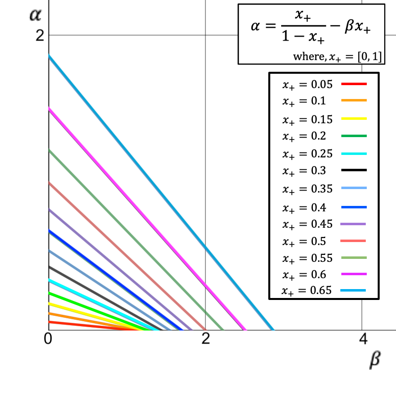
Thus, observing \(x_+\) does not allow for identification of the model parameters \(\alpha\) and \(\beta\). A solution to this issue would be to observe the value of \(x(t)\) at additional time points rather than only the equilibrium fraction. However, if the original parameters \(a\), \(c\) and \(N\) are unknown, even exact knowledge of the entire trajectory \(I(t)\) does not facilitate parameter identifiability. Although \(b\) can be determined from knowledge of \(I(t)\), at least one of the parameters \(\{a,c,N\}\) must be observed directly in order to identify the others.
While \(N\) is typically known in practice, knowing the population size alone does not resolve the identifiability issue here. The parameters \(a\), \(c\), and \(N\) enter the model only through their composite effect in \(b\), meaning that they remain structurally confounded even with perfect, error-free observations of \(I(t)\). This example therefore illustrates the broader point that identifiability depends on what is observed: richer or more granular data can break structural equivalences that remain hidden when only aggregated outcomes are available.
In particular, the identifiability problem can vanish if different or more informative outcomes are used as summary statistics, underlining how central this choice is for calibration.
In this example, we see that parameters may fail to be identifiable even in a simple deterministic model with perfect observations. Motivated by this, we next investigate how similar structural identifiability issues can arise in ABMs and how these may be exacerbated by agent heterogeneity.
Method
Experimental framework
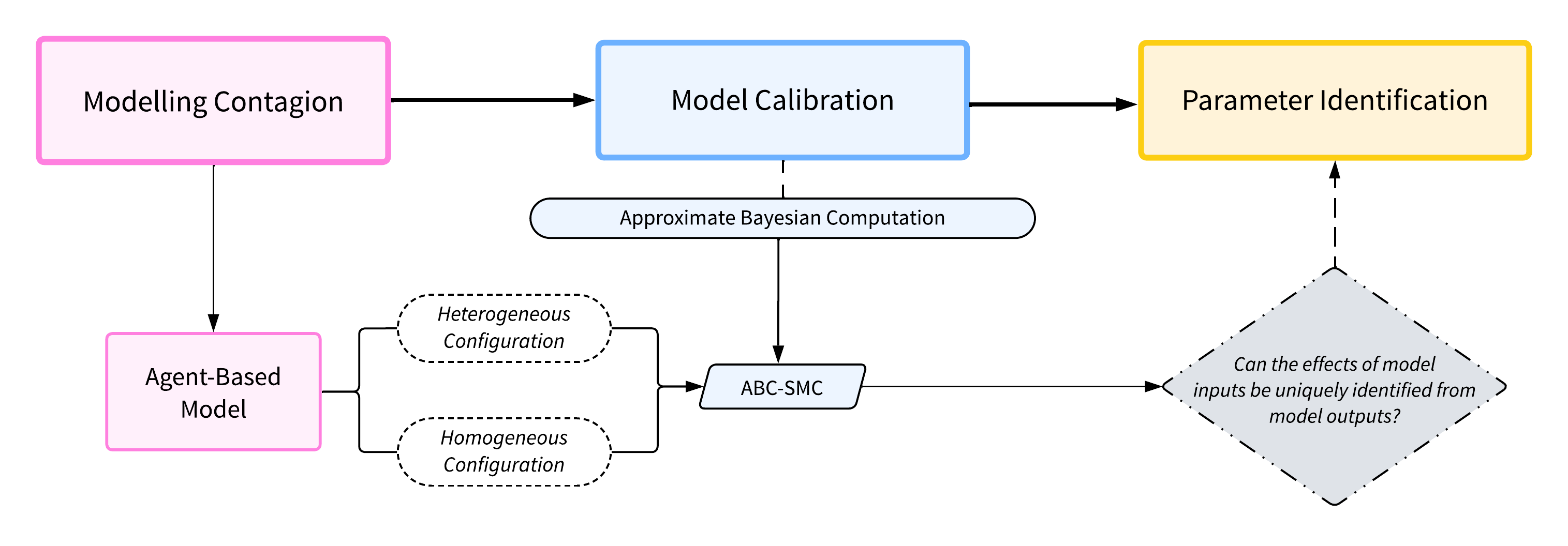
This study of parameter identification combines two main components: agent-based models (ABMs) and Approximate Bayesian Computation (ABC) calibration. This section summarises how these components are interconnected, with the workflow presented in Figure 21.
Motivated by the ODE example presented above, a contagion ABM was developed to facilitate a comparative study of homogeneous and heterogeneous scenarios, referred to as configurations in this study. A set of arbitrary (‘default’) ABM parameter values was selected to generate the ground truth data. ABC was then employed to calibrate the model. The primary focus of this study lies not on the calibration process itself, but on the application of ABC’s iterative resampling technique to explore the parameter space and use uncertainty as an indicator of parameter identifiability. The parameter values used in this study were informed by sensitivity analyses conducted on all key model parameters, which explored their influence on epidemic dynamics and calibration performance. These analyses guided the choice of representative values that illustrate parameter identifiability challenges while remaining computationally tractable.
The ABC procedure iteratively reduces the parameter space and moves toward combinations that best reproduce the observed data. In Bayesian inference, identifiability does not require the posterior to collapse to a single value; instead, a parameter is considered identifiable when its posterior mass concentrates sufficiently around the true value. Conversely, if ABC fails to uniquely determine these inputs, this suggests the presence of a parameter identification problem. To validate this, graphical illustrations of the homogeneous ODE model are used as references for the exhibited dynamics, enabling us to evaluate the presence or absence of parameter identification issues within the ABM configurations.
Simple contagion agent-based model
The simple contagion model presented here is based on the Susceptible-Infected-Susceptible-Spontaneous (SISa) model framework (Hill et al. 2010) and should be considered a toy model for demonstrative purposes only. The model simulates the process and spread of infectious diseases within an agent population.
Figure 3 summarizes the transmission of contagion into two states and three processes.
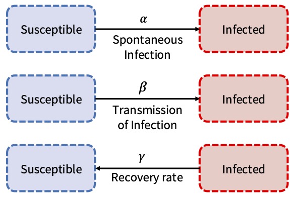
Agents occupy one of two states at the end of each time period (iteration): susceptible or infected. They can transition between these states according to the parameters \(\alpha\), \(\beta\) and \(\gamma\). The parameter \(\alpha\) denotes the background rate of infection, referring to the constant spontaneous rate of infection within the population, which transmits the infection to a susceptible agent regardless of the state of their contacts. The parameter \(\beta\) represents the inter-agent infection rate, which is the transmission rate of infection to susceptible individuals. The parameter \(\gamma\) is the recovery rate, representing the transition from the infected state back to the susceptible state, independent of the state of an agent’s contacts.
It is important to note that, as this ABM is non-spatial, agents interact indirectly, meaning they can observe each other’s states (whether susceptible or infected) during each iteration. Consequently, inter-agent contamination occurs randomly. An agent changes their state in response to the propensity \(\mathcal{P}\). To assess their condition, an agent compares their state to that of another randomly chosen agent, denoted as Agent\(_A\) (the assessing agent) and Agent\(_i\) (the reference agent). Agent\(_A\) determines their propensity of infection based on Agent\(_i\)’s state in the previous iteration. If Agent\(_i\) is susceptible, the propensity is determined only by the background infection rate, i.e., \(\mathcal{P} = \alpha\). If Agent\(_i\) is infected, the propensity includes both the background rate and an additional transmission factor, i.e., \(\mathcal{P} = \alpha + \beta\). If an agent is infected, their propensity to become susceptible is \(\mathcal{P}=\gamma\). An agent changes its state if \(\mathcal{P}>r\), where \(r\) is a uniformly generated random number on the interval \((0,1)\).
Homogeneous and heterogeneous model configurations
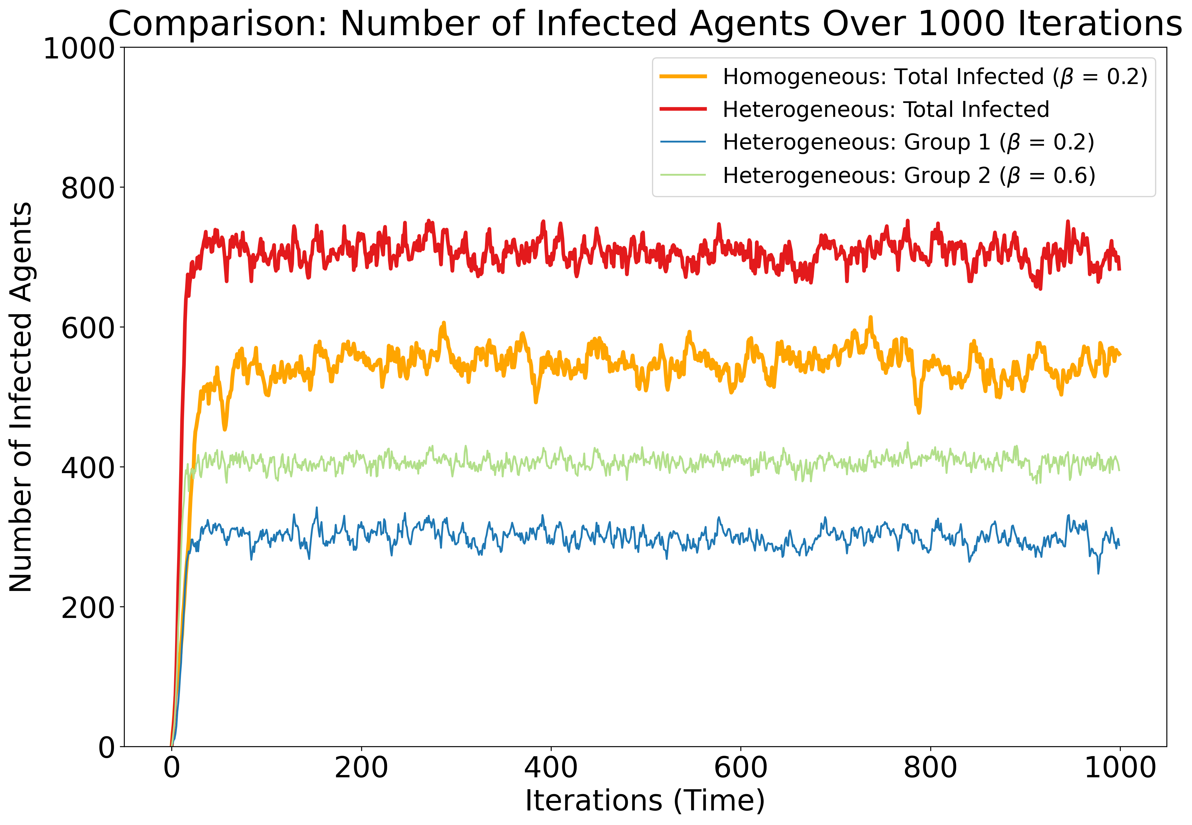
The case study model consists of two configurations: homogeneous and heterogeneous. In both configurations, agents share the same fundamental parameters and processes. In the homogeneous configuration, the agent population determines their propensities using the same fixed values for \(\alpha\) and \(\beta\), making all agents identical. Heterogeneity is then introduced by dividing agents into two groups, with propensities constructed using different values of \(\beta\) for each group, while the parameters \(\alpha\) and \(\gamma\) remain fixed. Table 1 outlines the default values used to initialise the model configurations. Figure 4 illustrates the model output from these configurations, which will serve as the ‘ground truth’ and be referred to as ‘observed data’ in subsequent analysis.
| Parameter | Homogeneous Config. | Heterogeneous Config. | |
|---|---|---|---|
| Number of Agents | 1000 | 1000 | |
| Iterations (Time, \(t\)) | 1000 | 1000 | |
| Number of Agent Groups | 1 | 2 | |
| Alpha (\(\alpha\)) | 0.01 | 0.01 | |
| Beta (\(\beta\)) | 0.2 | ||
| \(\beta_{\text{Group1}}\) | 0.2 | ||
| \(\beta_{\text{Group2}}\) | 0.6 | ||
| Gamma (\(\gamma\)) | 0.1 | 0.1 | |
Further, Figure 4 compares the infection dynamics over \(1000\) iterations in the homogeneous and heterogeneous agent-based models. The homogeneous configuration (orange) shows the total number of infected agents under a single transmission rate (\(\beta = 0.2\)). The heterogeneous configuration (red, blue, and green) introduces two agent groups with distinct transmission rates (\(\beta_{\text{Group1}} = 0.2\), \(\beta_{\text{Group1}} = 0.6\)), resulting in higher overall infection levels and distinct group-specific dynamics. The comparison highlights how introducing heterogeneity alters the aggregate epidemic trajectory and equilibrium state.
Sensitivity analysis
To complement the calibration results and provide a deeper understanding of how key parameters influence model behaviour, a sensitivity analysis was conducted. The aim was to examine how variation in the infection transmission rate (\(\beta\)), recovery rate (\(\gamma\)), and spontaneous infection rate (\(\alpha\)) affects the proportion of infected agents in the agent-based model.
For each experiment, a single parameter was systematically varied while the remaining two were held constant at specific values. There were 100 simulations, and each simulation involved 1000 agents over 100 iterations. The mean proportion of infected agents during the steady state (defined as the final 20% of iterations) was recorded. This approach isolates the marginal effect of each parameter and allows us to assess the model’s responsiveness across plausible parameter ranges.
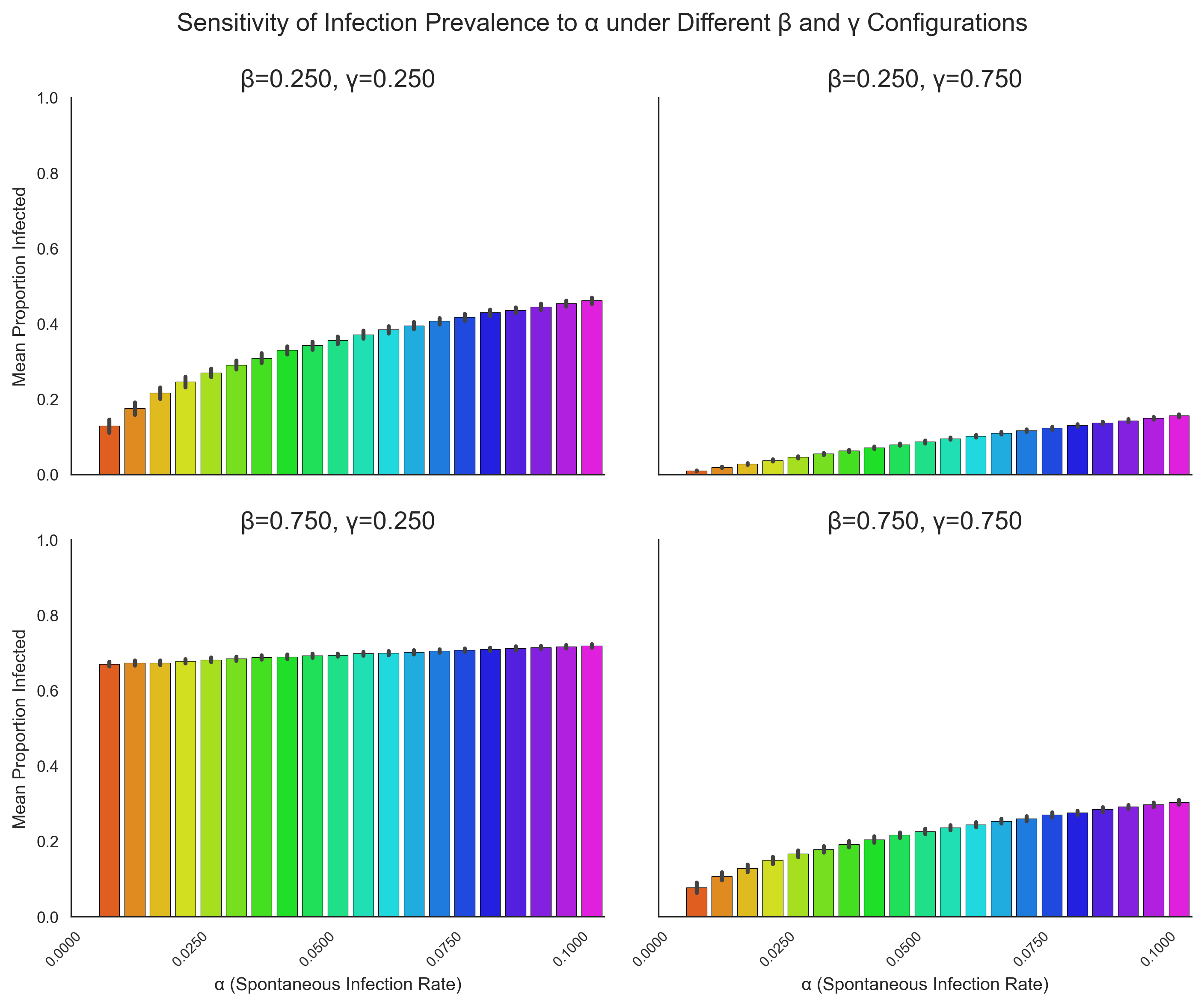
Figure 6 summarises the sensitivity of infection prevalence to the three parameters. Each panel shows the effect of varying one parameter while the remaining two are held fixed at four different combinations. Error bars represent the standard deviation across simulation replicates.
Transmission rate (\(\beta\)): The middle panel of Figure 6 shows how varying \(\beta\) from 0 to 1 influences infection dynamics under four combinations of \(\alpha\) and \(\gamma\) (0.25 or 0.75 for each). Across all cases, infection prevalence increases monotonically with \(\beta\), confirming its dominant role in driving epidemic spread. The steepness of this increase is modulated by \(\gamma\): higher recovery rates dampen the effect of \(\beta\), highlighting the interaction between transmission and recovery processes.
Recovery rate (\(\gamma\)): The right-hand panel of Figure 6 explores sensitivity to \(\gamma\) while \(\alpha\) and \(\beta\) are held constant. As expected, increasing \(\gamma\) reduces the mean proportion of infected agents. However, the magnitude of this effect depends on \(\beta\), with higher transmission rates requiring larger increases in \(\gamma\) to noticeably lower prevalence. Interestingly, because \(\gamma\) primarily rescales the time over which the dynamics unfold, its impact on the shape of epidemic curves can often be accounted for by adjusting the temporal axis rather than altering equilibrium outcomes.
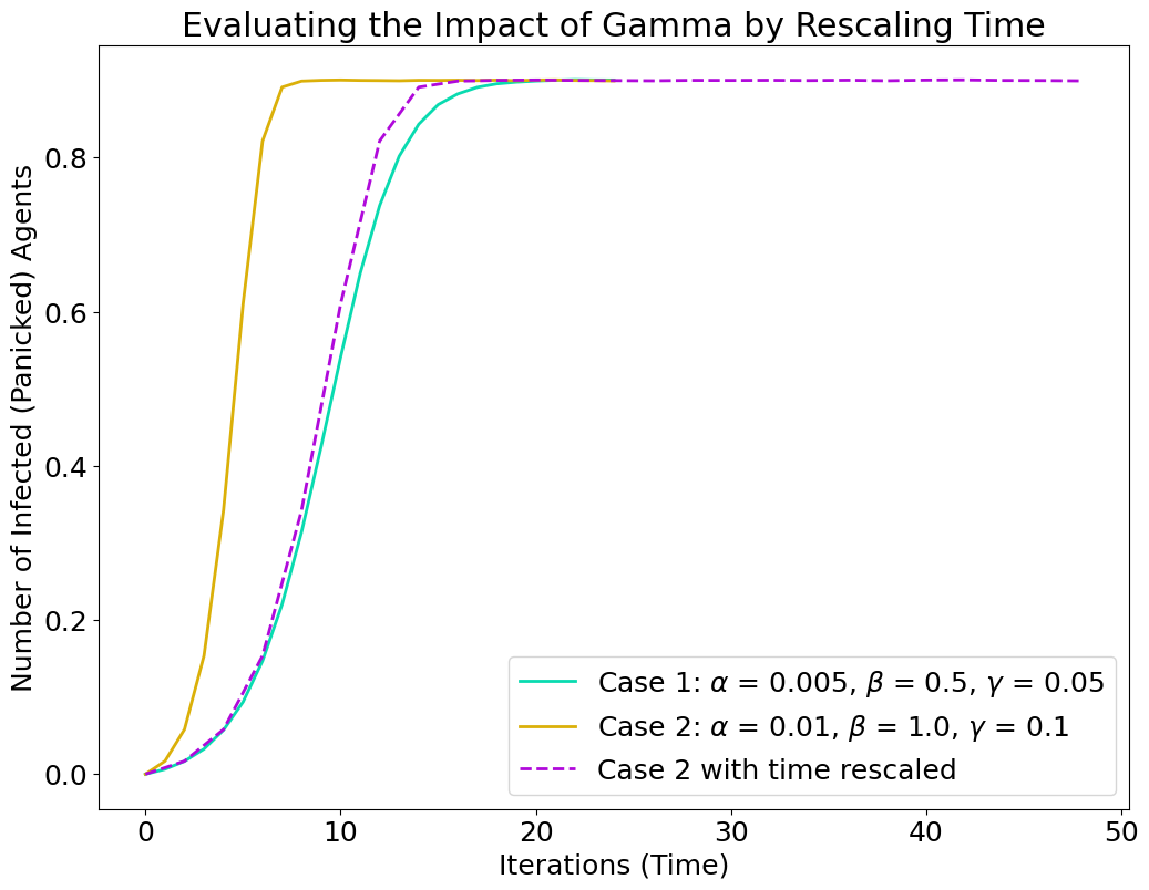
This property is illustrated in Figure 5, which compares two cases with different \(\gamma\) values. When time is rescaled, the infection curves overlap almost perfectly, indicating that \(\gamma\) primarily influences the pace rather than the qualitative nature of epidemic dynamics. For this reason, \(\gamma\) was held fixed in some subsequent analyses, allowing the sensitivity study to focus on parameters that shape equilibrium behaviour (\(\beta\) and \(\alpha\)).
Spontaneous infection rate (\(\alpha\)): The left-hand panel of Figure 6 examines sensitivity to \(\alpha\), varied between 0 and 0.1. Even within this relatively narrow range, small increases in \(\alpha\) noticeably affect infection prevalence, particularly when \(\beta\) is high. This reflects the disproportionate influence that rare spontaneous infections can have on the dynamics, as even low levels of external introduction are sufficient to sustain an outbreak under favourable transmission conditions.
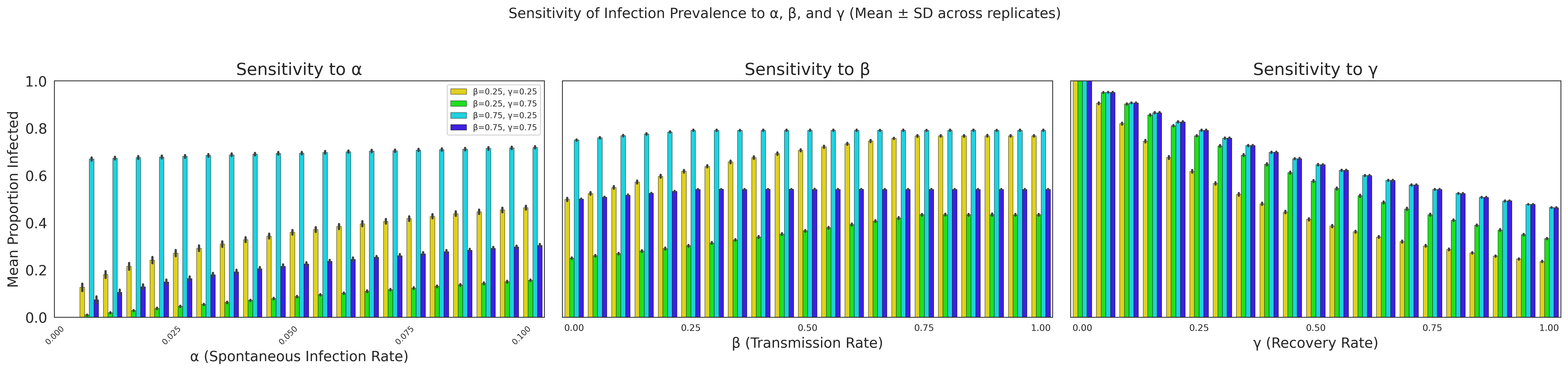
To illustrate this point more clearly, Appendix A presents the same analysis using larger values of \(\beta\) and \(\gamma\) (0.25 and 0.75 rather than 0.025 and 0.075). In this regime, the influence of \(\alpha\) becomes almost indistinguishable: the dynamics are dominated by transmission and recovery processes, and variations in \(\alpha\) produce only marginal changes in prevalence. This comparison supports the choice of smaller \(\beta\) and \(\gamma\) values in the main analysis, as it ensures that the effects of \(\alpha\) remain visible and that its identifiability can be meaningfully examined.
Together, these analyses demonstrate the sensitivity of epidemic outcomes to key parameters and underscore the importance of considering parameter interactions during calibration. They also reinforce the identifiability challenges discussed earlier: overlapping effects of \(\beta\), \(\gamma\), and \(\alpha\) mean that different parameter combinations can yield similar outcomes, complicating parameter inference from observed data.
These structural identifiability challenges are further compounded by the assumption that only the overall infection curve is observed. If it were possible to distinguish between spontaneous and non-spontaneous infections or to observe separate infection trajectories for the two agent groups, the parameters would become much more distinguishable. In such cases, identifiability would be considerably less challenging, highlighting how strongly the calibration process depends on the granularity of the available data.
Rationale for parameter choices
The parameter values used in the main analysis were selected to reflect qualitatively distinct but epidemiologically plausible regimes that make structural identifiability issues visible while keeping the model computationally tractable. Specifically, \(\beta = 0.2\) and \(\beta = 0.6\) were chosen to represent two transmission environments, one relatively low and one substantially higher, thereby introducing meaningful heterogeneity between agent groups without producing trivial epidemic outcomes (such as extinction or near-universal infection).
The recovery rate, \(\gamma\), was held constant to isolate the effects of transmission heterogeneity and to reduce the dimensionality of the parameter space, thereby focusing the analysis on the identifiability challenges associated with \(\beta\). Finally, \(\alpha\) was fixed at a small value (0.01), consistent with Table 1, to represent rare spontaneous infections that seed outbreaks without dominating the dynamics. Using substantially larger values of \(\beta\) and \(\gamma\) would have overwhelmed the influence of \(\alpha\), as demonstrated in Appendix A, making the parameter effectively indistinguishable. These modelling choices ensure that the effects of \(\alpha\) remain visible and allow the analysis to illustrate how even modest heterogeneity in transmission parameters can complicate parameter identification.
Approximate Bayesian Computation (ABC)
Approximate Bayesian Computation (ABC) is a method of Bayesian inference originally introduced in the biological sciences (Fu & Li 1997; Pritchard et al. 1999; Tavaré et al. 1997; Weiss & von Haeseler 1998). In Bayesian inference, the likelihood quantifies how well a set of model parameters explains the observed data. When the likelihood is known, the posterior distribution can be directly and continuously updated as new data become available (Beaumont et al. 2002). However, in more complex scenarios, deriving the likelihood function may be challenging or even infeasible. In such cases, ABC methods provide a practical alternative, approximating the posterior distribution using sampled data. For a detailed overview of the foundations of ABC, its algorithmic advancements, and its applications in fields such as evolutionary biology and ecology, Csilléry et al. (2010) offer a comprehensive review. For a recent overview of ABC, see Beaumont (2019).
In ABMs, likelihood functions are frequently intractable due to the complexity of the models. Recently, ABC has been proposed as an effective alternative for model calibration (Grazzini et al. 2017; Turner & van Zandt 2012). Various ABC algorithms have been applied in the literature (Beaumont et al. 2002; Beaumont 2010; Hartig et al. 2011; Martínez et al. 2011; May et al. 2013; Sottoriva & Tavaré 2010; Thiele et al. 2014; Toni et al. 2009; Zbair et al. 2023), with the most common being rejection sampling and sequential Monte Carlo.
ABC methods have been used to calibrate ABMs. Their capacity to evaluate uncertainty in individual parameter estimates and their iterative approach, provides substantial potential for revealing new insights (Grazzini et al. 2017; Toni et al. 2009). However, as noted earlier, our use of ABC diverges from its conventional application. In this study, ABC is utilised to explore the parameter space and interpret uncertainty as an indicator of parameter identifiability.
The sensitivity analysis presented here focuses on the model parameters themselves. A systematic sensitivity analysis of the full ABC-SMC pipeline (including alternative priors, tolerance schedules, distance metrics, or summary statistics) lies beyond the scope of this study. Importantly, however, the identifiability issues we observe arise from the structure of the model and the limited informativeness of the aggregated infection curve, rather than from specific ABC hyperparameter settings. Our aim is not to optimise the ABC procedure but to use it as a diagnostic tool to reveal when the available data are insufficiently informative to distinguish between parameter values.
We will briefly outline the Approximate Bayesian Computation Sequential Monte Carlo (ABC-SMC) method. For further detail, the interested reader can refer to the tutorial by Turner & van Zandt (2012). ABC-SMC was implemented using the Python package, pyABC (Schälte et al. 2022).
The posterior distribution, \(\pi(\theta\mid Y)\), of a set of model parameters \(\theta\) given observed data \(Y\), can be computed from the likelihood \(\mathcal{L}(Y\mid\theta)\) of observing the data \(Y\) given the parameters \(\theta\), and a prior distribution for the parameters \(\pi(\theta)\), since Bayes theorem tells us that
| \[\pi(\theta\mid Y) \varpropto \mathcal{L}(Y \mid\theta)\pi(\theta).\] | \[(5)\] |
In cases where the likelihood cannot be evaluated directly, ABC provides a likelihood-free approximation to the posterior. Instead of computing \(\mathcal{L}(Y \mid\theta)\), ABC relies on simulating data under proposed parameter values and retaining those simulations that are sufficiently close to the observed data. This leads to the approximate posterior
| \[\pi_{\epsilon} (\theta\mid Y) \varpropto \int K_{\epsilon}(\rho(Y, X)) \pi(\theta)p(X \mid \theta)dX.\] | \[(6)\] |
ABC operates by generating a sample of candidate parameter values, denoted as \(\theta^{*}\), and using these to produce simulated data, \(X\). In this study, the contagion ABM is employed to generate \(X\) by running the model with \(\theta\) as input parameter values. The distance between the observed data (\(Y\)) and the simulated data (\(X\)), denoted as \(\rho (Y, X)\), determines whether \(\theta\) is retained. ABC assigns a weight, (\(w\)), to each particle according to \(\rho(Y, X)\). This distance is calculated using the Root Mean Square Error (RMSE), calculating the numerical difference between ground truth and the simulated Number of Infected agents.
From this, the posterior distribution is made up of parameter samples (called ‘particles’ in pyABC terminology) with the smallest distances. In each iteration, the particles are re-sampled and their weights are re-calculated until the Number of Iterations has been satisfied. Although RMSE is a common distance metric in ABC applications, it can be sensitive to outliers. Alternative metrics such as the mean absolute error (MAE) or Wasserstein distance could, in principle, capture different aspects of the discrepancy between observed and simulated data (Bernton et al. 2019; Jiang et al. 2015). A full sensitivity analysis of the ABC-SMC hyperparameters (tolerance schedule, priors, distance metrics) concerns practical identifiability and lies beyond the scope of this study, which focuses on structural identifiability arising from the model and summary statistics.
In the present setting, however, the identifiability challenges arise because distinct parameter combinations produce very similar infection trajectories under the chosen summary statistics. As a result, switching to a different distance metric would not substantially change the qualitative behaviour of the posterior in this case; the limitation stems from the informativeness of the summaries rather than from the particular choice of metric. Figure 7 illustrates the SMC process.
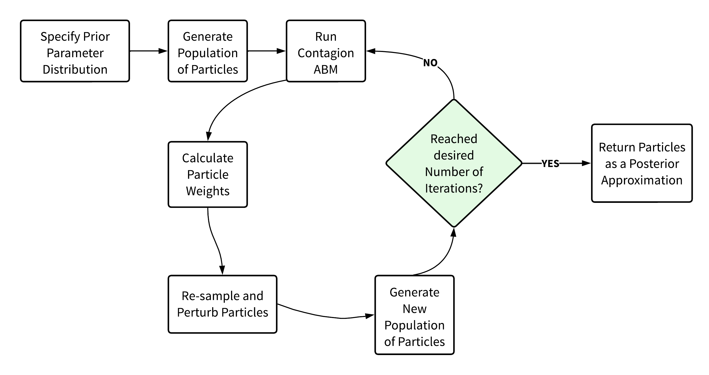
Table 2 summarises the parameters used to initialise the pyABC algorithm. In Table 2, Observed Data (\(Y\)) refers to the “true” data against which pyABC’s simulated data (\(X\)) is compared, while the summary statistic represents a reduced representation of that simulated data used by the ABC-SMC algorithm for parameter inference. The distinction is important: while \(Y\) provides the empirical or ground-truth reference for calibration, the summary statistic condenses the essential features of \(X\) into a form that is informative for the inference process.
An important modelling decision concerns the choice to represent the observed data, \(Y\), using the cumulative distribution function (CDF) of the number of infected agents rather than a simple temporal series or a single scalar summary such as the mean. The CDF captures the full distributional dynamics of the epidemic process over time, rather than relying solely on point estimates such as final infection levels. This provides a richer and more informative basis for parameter inference in the ABC-SMC framework, as the CDF reflects both the magnitude and the temporal evolution of infections.
To compute the CDF, the number of infected agents at each time step in the observed data is sorted, and the cumulative proportion of infected agents is calculated and normalised by the total population size. This yields a monotonic cumulative curve that summarises the distribution of infection levels across the entire simulation. Although pyABC uses the average number of infected agents as the summary statistic for parameter inference, the observed data were represented using the CDF to increase the amount of information available for comparison and to highlight identifiability issues arising from the structure of the model. The intention was to ensure that any remaining identifiability problems were due to the model–parameter relationship itself rather than to limitations in how the data were represented.
This modelling decision also illustrates a broader methodological point raised in the literature: parameter identifiability is shaped not only by the structure of the model but also by the structure and informativeness of the data provided to the calibration algorithm (Wieland et al. 2021). Transforming model outputs into a cumulative distribution rather than a single scalar value increases the amount of information available to pyABC and can improve its ability to distinguish between competing parameter sets. While richer data representations and alternative summary statistics could further influence identifiability, the focus of this study is on structural identifiability, that is, challenges inherent to the model’s formulation and parameter interactions, rather than practical identifiability problems that stem from data limitations. Our results show that even when using standard calibration settings (e.g. average number of infected agents), identifiability challenges persist as a property of the model–parameter relationship itself.
| Parameter | Model Configuration |
|---|---|
| Observed Data, \(Y\) | CDF (Number of Infected) |
| Summary Statistic of \(X\) | Average Number of Infected |
| Distance Function | RMSE |
| Max Number of Population | 12 |
| Population Size (No. of Particles) | 1000 |
| \(\alpha\) | \(\mathcal{U}\) (0.0, 0.1) |
| \(\beta_{\text{Group 1}}\) | \(\mathcal{U}\) (0.0, 1.0) |
| \(\beta_{\text{Group 2}}\) | \(\mathcal{U}\) (0.0, 1.0) |
The task of the ABM-SMC algorithm is to estimate the model parameter values (\(\alpha\) and \(\beta\)) that are most likely to produce simulation data that is close to the ground truth. ABC-SMC begins by sampling the model parameters from a prior distribution, which in this case is uniformly distributed so that every possible parameter value between \(0\)-\(1\) has an equal chance of occurring. ABC-SMC needs \(n\) particles to search the parameter space, where each particle is a sample of the model parameter values from the prior distribution and runs the case study model.
The algorithm has two stopping functions, Maximum Number of Population and Epsilon (\(\epsilon\)). Considering the aim of our use case is to minimise the root mean square error (RMSE) between the observed case study data and simulated pyABC data, reaching \(\epsilon = 0\) is infeasible because of model stochasticity. Instead, we use the Max. Number of Population as the stopping criterion, meaning the number of sample populations is fixed, and each sequentially improves on the posterior approximation, while keeping the computational time feasible.
Selecting an appropriate population size is case-dependent and it is difficult to give useful general guidelines (Del Moral et al. 2012). However, it is understood that too small of a population size yields large approximation errors, which hampers convergence, while too large a population size results in an unnecessary computational burden (Klinger & Hasenauer 2017). This paper will consider the Max. Number of Populations typically used in pyABC examples as default, this number is \(10\) but will explore a further \(2\) generations to investigate whether the additional generations improved model performance. Therefore, the Max. Number of Populations will be fixed at \(12\).
Once the Max. Number of Populations has been reached, the posterior distribution is estimated using each successful particle’s parameter values. Posteriors can be further improved by rerunning ABC-SMC using the estimated posterior distribution. To assess the success and quality of PyABC calibration, alongside each posterior distribution, the Maximum a-Posteriori Probability (MAP) estimate or posterior mode, summary statistic and credibility intervals will be presented.
Results
In this section, we will present the calibration results of the contagion ABM. As the focus of this study is not pyABC itself but rather the iterative resampling technique we will use to explore the parameter space. From this, we demonstrate the presence of structural identification issues in ABMs. Furthermore, this section will also consider the potential implications of these unresolved structural identification issues.
PyABC for parameter identification: An agent-based model illustration
Case study: Homogeneous configuration
For the homogeneous model, we aim to estimate the infection rate parameters \(\alpha\) and \(\beta\) by calibrating the agent-based model introduced in Section 4.3 against observed data \(Y\). Parameter values are drawn from the prior distributions specified in Table 2, and the resulting simulated data \(X\) are compared with \(Y\) using the distance metric described in Section 4. Parameter samples that minimise this distance are accepted into the posterior distribution. For the homogeneous run, we used independent priors \(\alpha \sim U(0, 0.1)\) and \(\beta \sim U(0, 1)\); for the heterogeneous run, \(\beta_{\text{Group1}},\, \beta_{\text{Group2}} \sim U(0, 1)\), as in Table 2.
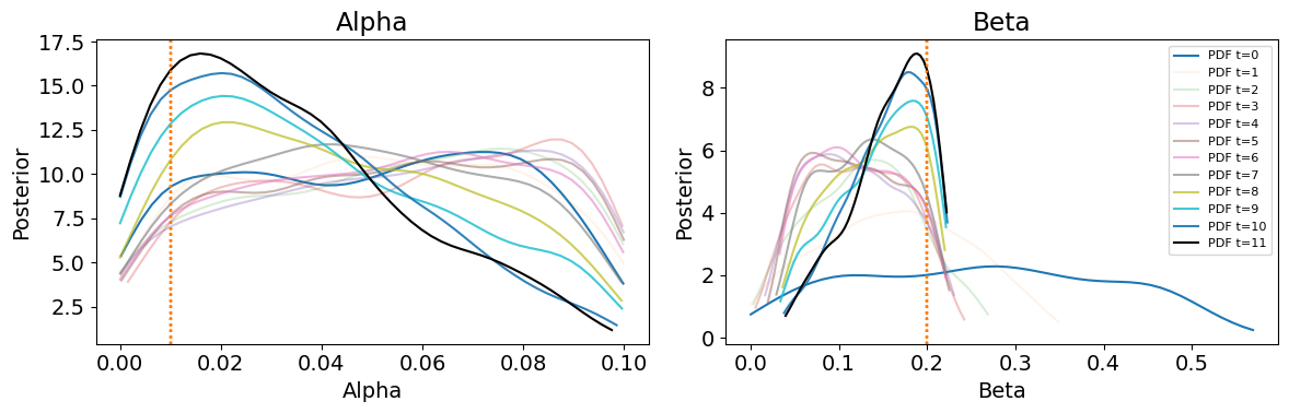
Through the sequential Monte Carlo process, parameter distributions are iteratively updated to reduce the discrepancy between the simulated and observed data. Calibration proceeds until the maximum number of populations (\(T = 11\)) is reached, at which point the final posterior represents the most refined approximation of the parameter distributions, associated with the smallest tolerance, \(\epsilon\). Kernel density estimates of the posterior marginal distributions for \(\alpha\) and \(\beta\) are presented in Figure 8, with corresponding marginal posterior modes (MAP estimates) and credibility intervals for each distribution in Table 6.
| Parameter | True Values | Posterior Modes | 95% CI |
|---|---|---|---|
| \(\alpha\) | 0.01 | 0.01595468 | 0.0013, 0.0740 |
| \(\beta\) | 0.2 | 0.18851214 | 0.0828, 0.2169 |
| Summary Stat: Average | 534 | 535 | |
The true values of \(\alpha\) and \(\beta\) are indicated by the dashed vertical lines in Figure 8 and summarised in Table 3. Although these true values do not exactly coincide with the peaks of the marginal posteriors (MAP estimates), they lie in close proximity. This indicates that if the marginal posterior modes were used to initialise the case study ABM, the resulting model output would closely approximate the observed data. In other words, the calibration process has successfully narrowed the parameter space to a region consistent with the empirical dynamics.
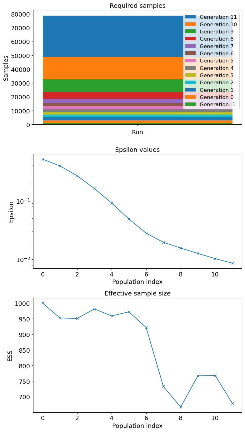
Once pyABC completes its iterative process, it produces a final posterior distribution at \(T = 11\) containing the accepted particles. However, pyABC indexes populations from \(T = 0\), meaning the calibration produces a total of 12 populations, each representing a progressively refined approximation of the posterior distribution.
Convergence diagnostics for the homogeneous case are shown in Figure 9, which illustrates the decline in RMSE and its dispersion (IQR) across successive pyABC populations, indicating that the algorithm is progressively approximating the target distribution. Additional diagnostics, including the evolution of the tolerance \(\epsilon\) and the Effective Sample Size (ESS), are provided in Appendix B, further confirming that the posterior uncertainty observed here is not primarily due to premature termination of the pyABC process.
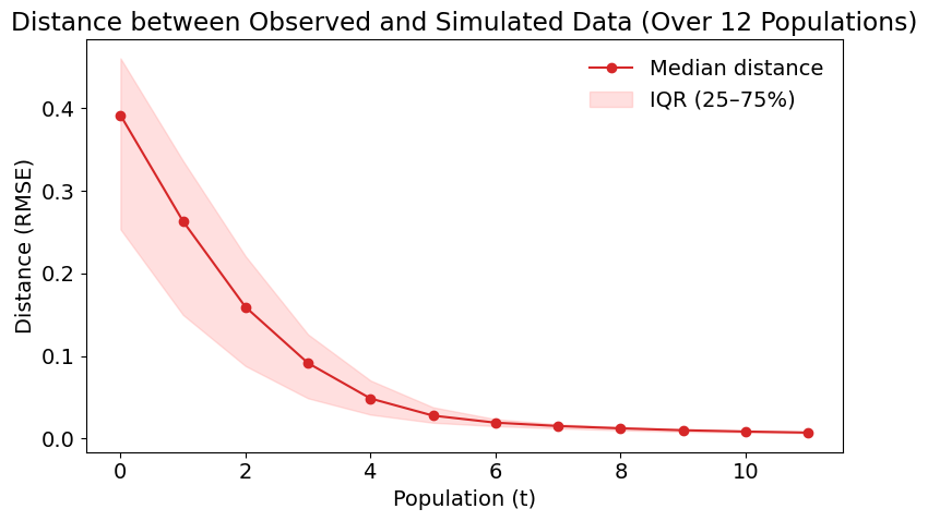
Figure 10 illustrates the evolution of the posterior distribution throughout the pyABC calibration process for the homogeneous model. The figure uses a density plot in which lighter regions indicate higher concentrations of accepted particles, representing parameter combinations that more frequently reproduce the observed dynamics. Conversely, darker regions correspond to sparse or low-support areas where accepted particles are less common. As the populations progress, the distribution becomes increasingly concentrated, reflecting the algorithm’s movement toward parameter combinations that better match the observed data.
The plot also displays two reference points: the green dot marks the true parameter values used to generate the observed data, and the red dot indicates the posterior mode in the final population. As the calibration advances, the density shifts toward the region surrounding the true values, and by the final population, the posterior mode sits near the green truth marker. The overall contraction of the high-density regions, along with the convergence of the red dot toward the green dot, demonstrates that both \(\alpha\) and \(\beta\) are identifiable in the homogeneous configuration, with the posterior narrowing around a consistent set of parameter values. Notably, the final posterior distribution (T = \(11\)) presents a linear relationship consistent with the dynamics uncovered in the ODE contagion model (Figure 1), reinforcing the structural origins of the identifiability issue.
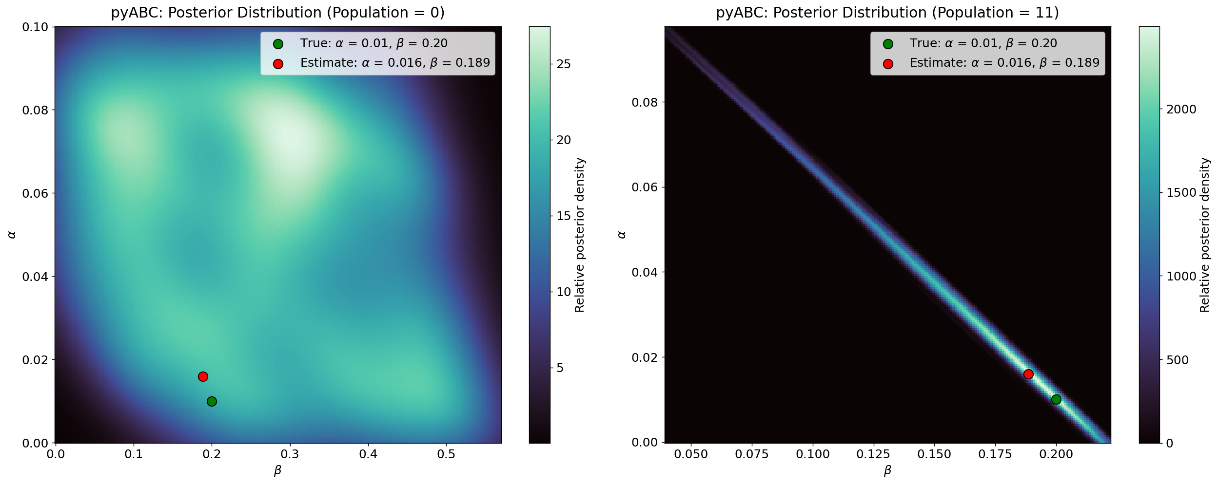
The final posterior distribution (T = \(11\)) also reveals an important feature of the calibration process. Each posterior distribution consists of approximately \(1000\) accepted particles, combinations of \(\alpha\), \(\beta\) parameter, each of which generates simulated data whose cumulative distribution closely approximates the observed data. These accepted parameter combinations are visualised in Figure 11, where each dot represents a particle from the final posterior population.
The fitted line in Figure 11 illustrates the functional relationship between \(\alpha\) and \(\beta\) implied by the calibration: a continuum of parameter combinations along this trajectory can reproduce the same equilibrium behaviour in the ABM. This structure reflects the underlying identifiability issue, multiple parameter sets yield indistinguishable model outputs, yet the posterior weights provide additional information that peaks near the posterior modes, indicating that the data and summary statistic contain enough information to constrain the parameter space.
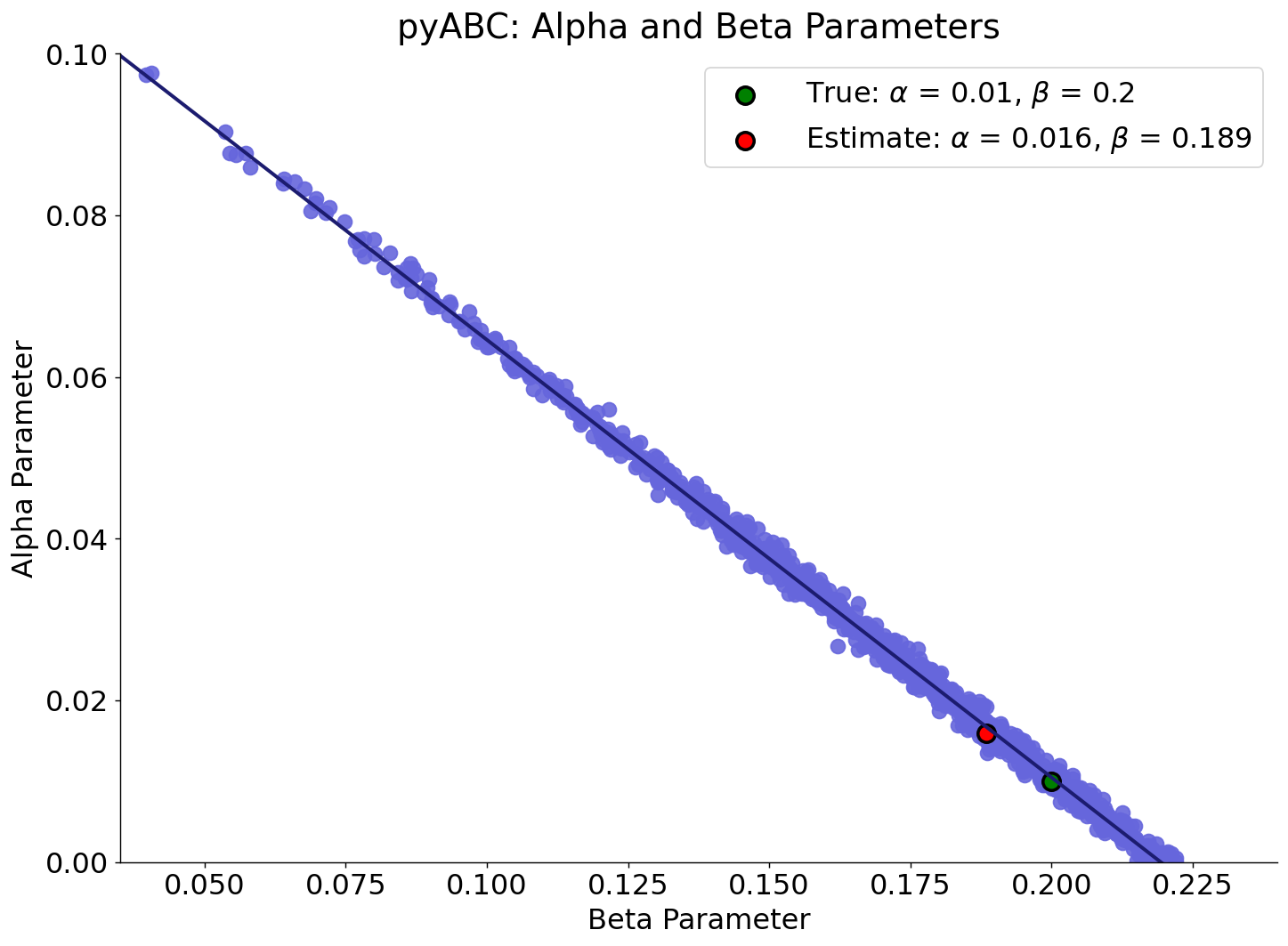
When comparing the true parameter values with the posterior modes and the summary statistic, the values are not exact but are reasonably close, and the true values lie within the \(95\%\) credibility intervals. However, the intervals themselves are relatively wide, indicating that while the calibration process has been successful in narrowing the parameter space, a broad range of plausible values remains. This demonstrates that the posterior modes provide a robust general estimate rather than a highly precise one.
Overall, this exercise demonstrates model calibration using ABC to determine posterior distributions for \(\alpha\) and \(\beta\) from a parameter space. pyABC produces credible estimates of the homogeneous configuration parameters, indicating structural identifiability under the chosen model-data relationship. This sets the stage for the subsequent section, which explores whether introducing heterogeneity through additional \(\beta\) parameters affects the quality of calibration and the degree of identifiability.
Case study: Heterogeneous configuration
In this study, heterogeneity refers specifically to agent granularity, introduced through an additional agent group with a distinct infection rate parameter, \(\beta_{\text{Group2}}\), alongside \(\beta_{\text{Group1}}\). This modification increases the dimensionality of the parameter space and provides an opportunity to investigate how introducing heterogeneity affects parameter identifiability.
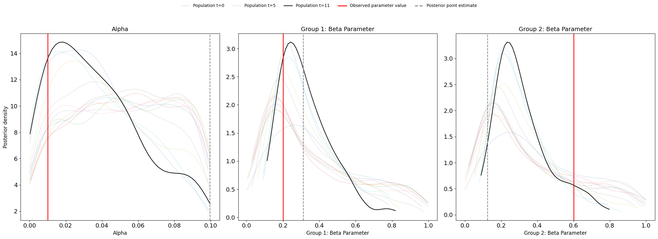
As in the homogeneous case, pyABC iteratively refines parameter estimates by minimising the distance between the observed data and the simulated data generated by the agent-based model. Figure 12 shows the posterior marginal distributions for \(\alpha\), \(\beta_{\text{Group1}}\), and \(\beta_{\text{Group2}}\). The posterior modes and \(95\%\) credibility intervals are summarised in Table 7, as well as pyABC output on epsilon and required samples in Figure 18.
Although the posterior peaks remain close to the true parameter values for \(\alpha\) and \(\beta_{\text{Group1}}\), the marginal distributions are substantially wider than in the homogeneous case. This reflects the additional uncertainty introduced by the second transmission parameter, \(\beta_{\text{Group2}}\). Notably, while \(\beta_{\text{Group1}}\) concentrates around a value close to its true parameter, \(\beta_{\text{Group2}}\) shifts toward much lower values, indicating that the observable data do not provide enough information to recover its true effect. Table 4 summarises these posterior modes and credible intervals.
| Parameter | True Values | Posterior Modes | 95% CI |
|---|---|---|---|
| \(\alpha\) | 0.01 | 0.01850757 | 0.0024–0.0856 |
| \(\beta_{\text{Group1}}\) | 0.2 | 0.24232129 | 0.1698–0.5550 |
| \(\beta_{\text{Group2}}\) | 0.6 | 0.23383305 | 0.1640–0.5718 |
| Summary Stat: Average | 700 | 699 | |
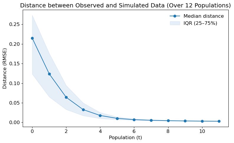
For the heterogeneous case, Figure 13, which tracks the reduction of RMSE and its interquartile range across pyABC populations. The decreasing trend confirms that the calibration process continues to learn from the data rather than stalling. Additional diagnostics in Appendix B, including the evolution of \(\epsilon\) and the Effective Sample Size (ESS), demonstrate that the remaining posterior uncertainty is structural rather than due to insufficient convergence of the algorithm.
Figure 14 illustrates the evolution of the joint posterior distribution over successive pyABC populations using a heatmap representation. Compared with the homogeneous case, the accepted particles in the heterogeneous configuration occupy a much broader region of the \((\beta_{\text{Group1}}, \beta_{\text{Group2}})\) parameter space. Crucially, the high-density regions do not contract around the true value of \(\beta_{\text{Group2}}\); instead, they shift toward much lower values. This explains why the posterior mode (red) point lies far from the true (green) value. By contrast, density remains more concentrated around the true \(\alpha\) and \(\beta_{\text{Group1}}\) values. The dispersion and displacement of the high-density regions indicate reduced identifiability introduced by the second transmission parameter: multiple combinations of \(\beta_{\text{Group1}}\) and \(\beta_{\text{Group2}}\) yield nearly indistinguishable infection trajectories, causing \(\beta_{\text{Group2}}\) to collapse toward \(\beta_{\text{Group1}}\) rather than recover its true value.
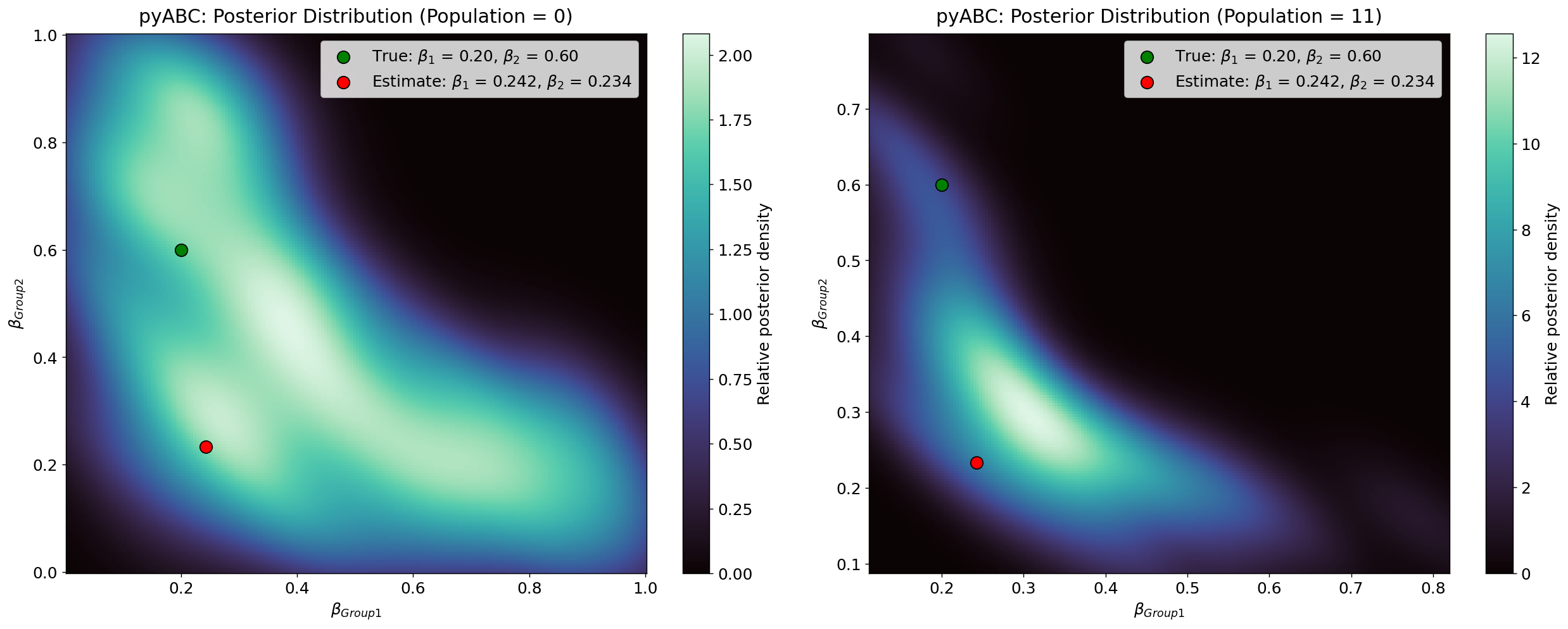
Further insights into parameter identifiability are provided by Figure 15, which shows the \(1000\) accepted parameter combinations from the final posterior population \((T = 11)\). Each point represents a pair (\(\beta_{\text{Group1}}\), \(\beta_{\text{Group2}}\)) that produced simulated data sufficiently close to the observed cumulative distribution. The green dot marks the true values used to generate the observed data, while the red dot indicates the posterior mode, representing the most frequently supported parameter combination in the final population.
Unlike the roughly linear \(\alpha\)-\(\beta\) structure seen in the homogeneous case, the accepted particles in the heterogeneous configuration form a curved, non-linear band across the parameter space. This dense band shows that many different (\(\beta_{\text{Group1}}\), \(\beta_{\text{Group2}}\)) pairs yield nearly indistinguishable infection trajectories under the available summary statistics. The high concentration of points near \(\beta_{\text{Group1}} \approx 0.24\) and \(\beta_{\text{Group2}} \approx 0.23\), combined with the displacement of the red posterior mode dot away from the green truth marker, indicates that \(\beta_{\text{Group2}}\) is not recoverable: its estimated value collapses toward \(\beta_{\text{Group1}}\), rather than remaining near its true value of \(0.6\). This pattern reflects a clear structural identifiability issue, where the two transmission parameters cannot be uniquely distinguished from the aggregate infection curve.
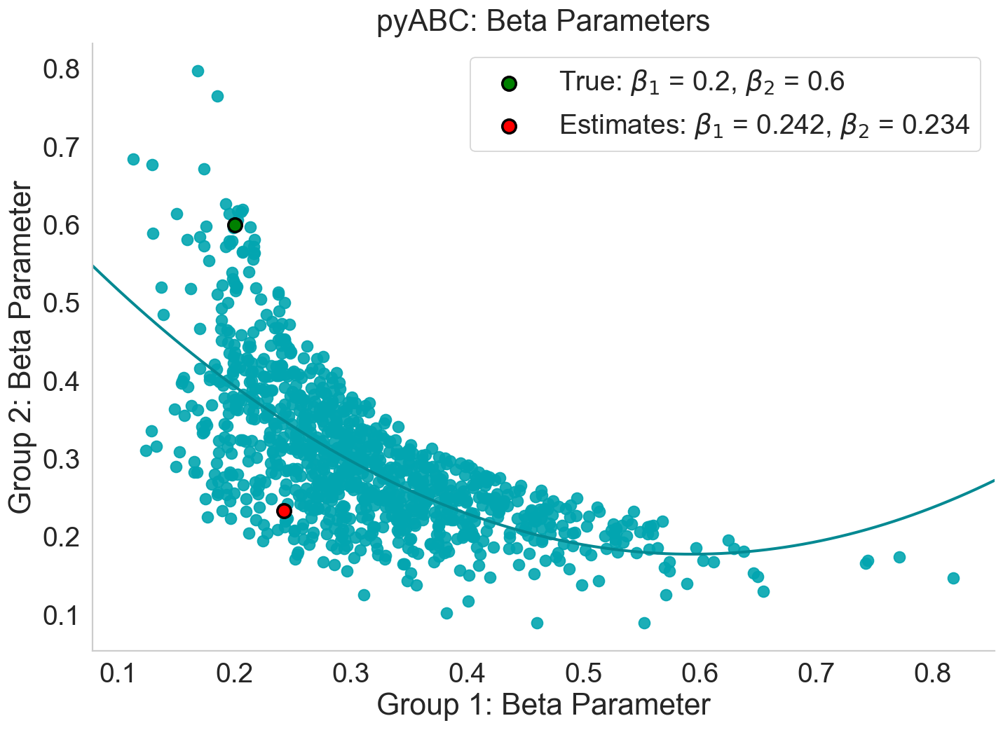
This pattern confirms that multiple combinations of \(\beta_{\text{Group1}}\) and \(\beta_{\text{Group2}}\) generate infection trajectories that are effectively indistinguishable when only the aggregate infection curve is used for calibration. Although pyABC successfully reduces the discrepancy between simulated and observed data, the algorithm is unable to uniquely attribute the observed dynamics to the individual contributions of the two transmission parameters. As a result, the posterior contracts toward a region where \(\beta_{\text{Group1}}\) and \(\beta_{\text{Group2}}\) take similar values, rather than recovering the true \(\beta_{\text{Group2}}\) value of \(0.6\). This demonstrates a clear structural identifiability issue: the additional heterogeneity introduced by a second \(\beta\) parameter increases the dimensionality of the model without providing sufficient observable information to separate their effects. Consequently, while the heterogeneous configuration increases descriptive realism, it simultaneously reduces the recoverability of the underlying parameters.
Discussion
Although the example above is hypothetical and simplified, it highlights a critical issue in ABM research: parameter identification. While only one parameter set and calibration run were presented in the main analysis, robustness checks (see Appendix C) indicate similar identifiability challenges across other configurations. Appendix C reports additional experiments in which heterogeneity was expressed in \(\alpha\) rather than \(\beta\), and in which the \(\beta\) parameters were numerically closer.
In all these cases, identifiability issues persisted, confirming that the problems highlighted in this study are not artefacts of a particular parameterisation. This was further illustrated in the heterogeneous configuration, where introducing a second infection parameter, \(\beta_{\text{Group2}}\), substantially increased model complexity and resulted in broader posterior distributions. Although calibration successfully reduced the distance between simulated and observed data, pyABC could not uniquely distinguish between the two \(\beta\) parameters, with many parameter combinations producing similar epidemic dynamics. This illustrates how even modest increases in model complexity can exacerbate structural identifiability issues, despite calibration appearing successful.
A further point concerns the type of observational data available. The identifiability issues shown here are partly a consequence of working only with the total infection curve. If spontaneous infections were observed separately, or if infection trajectories could be disaggregated by group, these outcomes would provide considerably more information for distinguishing between parameter values. In such cases, the overlap between trajectories generated by different parameter combinations would diminish, and identifiability would improve correspondingly.
This underlines that identifiability is shaped not only by the structure of the model but also by the informativeness of the summary statistics used for calibration. Increasing model complexity alone does not guarantee better empirical grounding if the observational data, or the chosen summaries, remain too coarse to retain the distinctions induced by different parameters. In principle, using separate CDFs for each group would retain more information about group-level transmission parameters and would substantially reduce the identifiability issues illustrated here.
Uncovering identification issues is just as essential as conducting sensitivity analyses, with each process reinforcing the other. We did not explore alternative methods for selecting summary statistics (e.g., PCA, neural networks), but these remain promising directions for future work. We also examined whether varying the proportion of agents across groups altered infection dynamics. The effective transmission rate \(\hat{\beta}\) can be expressed as a weighted average of group-specific parameters (derivation in Appendix C. Appendix C shows that infection levels depend primarily on the group with the larger population share, not necessarily the group with the higher \(\beta\) value. Relying only on the total infection curve, as done here, limits the ability to distinguish parameters; richer statistics, such as spontaneous-infection trajectories or group-specific CDFs, may improve identifiability.
To support practitioners, we suggest a simple checklist for assessing parameter identifiability during ABM calibration in a Bayesian framework:
| Step | Guidance |
|---|---|
| 1 | Compare posterior vs. prior – check whether the posterior reflects genuine learning from the data or largely reproduces the prior. |
| 2 | Inspect discrepancy distributions – examine the spread of accepted distances (e.g., RMSE) to distinguish structural non-identifiability from poor algorithmic convergence. |
| 3 | Evaluate summary statistics – ensure chosen statistics are sensitive to parameter variation; consider variance heuristics or dimension-reduction methods (e.g., PCA). |
| 4 | Replicate calibration runs – repeat the procedure with different random seeds or initialisations to confirm robustness of results. |
| 5 | Interpret wide posteriors cautiously – remember that they may reflect weak priors or limited convergence as well as structural non-identifiability. |
Note. Posterior contraction, the degree to which the posterior narrows relative to the prior, indicates how strongly the data inform the model. Simulation-Based Calibration (SBC) offers an additional diagnostic for assessing whether the inference procedure correctly recovers generating parameters, although it can be computationally demanding in ABC–SMC settings. For more on SBC, see Talts et al. (2018; Stan Development Team 2025).
These guidelines provide a starting point, but as the literature shows, identification problems remain widespread. Failure to correctly identify parameters in ABMs is common, but these issues can often be detected through cross-validation tests, as demonstrated by Carrella (2021). In their comparison of nine parameter estimation algorithms across 41 models, they found that no single algorithm consistently outperformed the others across all or even most models.
Resolving identification issues analytically remains challenging, even for mathematically tractable systems, and is even less straightforward for complex, stochastic ABMs. These challenges resonate with the broader debate between KISS (‘Keep It Simple, Stupid’) and KIDS (‘Keep It Descriptive, Stupid’) modelling strategies: as descriptive realism increases, tractability and identifiability often decrease. For such models, it is essential to explicitly acknowledge and document the influence of identification on the modelling process, as well as how these issues have been recognised and addressed (Guillaume et al. 2019).
Given the stochastic nature of ABMs, uncertainty is inherently present in the simulation process. However, when calibrating a model using chosen algorithms, repeated runs should not return vastly different parameter estimates. While this may seem trivial, modellers should systematically repeat the calibration process with various initialisations, ideally selecting random initial parameter values, to ensure that parameter estimates converge consistently (Shin et al. 2015).
ABMs are microscale models designed to simulate the interactions of multiple agents, often to replicate dynamics observed in real-world systems (Gustafsson & Sternad 2010). However, there has been increasing discussion on the potential for ABMs to serve as predictive tools (Chattoe-Brown 2023). If a model is structurally unidentifiable, it cannot be used for reliable predictions. Failing to uniquely determine input parameters from output data during estimation or calibration leads to inaccurate predictions, as key system behaviours may not have been captured during model development (Williams 2011). This issue has fuelled an ongoing debate in the ABM literature about the predictive utility of such models (Elsenbroich & Polhill 2023).
Polhill et al. (2021) identified path dependency as a key factor contributing to inaccuracies in ABM predictions, highlighting the intractability of exhaustively searching the space of models that could match the available data. They emphasised that while prediction is one possible use of ABMs, even inaccurate predictions can still provide value by identifying transitions between states in real-world systems.
While non-identification typically indicates a lack of sufficient information to distinguish between alternative models, in practice, obtaining the “right” information may take considerable time—or may never be possible at all (Rothenberg 1971). In some cases, having multiple plausible models may not pose significant issues, as differences in their predictions may be small enough to be acceptable or manageable through adaptive decision-making.
Regardless of how identification issues are handled, modellers have a responsibility to be transparent about the sources of these issues and how they were addressed. They should document whether model parameters were parametrically identified and how identifiability was assessed. If parameters were found to be non-identifiable, the documentation should also describe the anticipated consequences and any steps taken to mitigate them.
As demonstrated in the heterogeneous case, the posterior mode for \(\beta_{\text{Group2}}\) collapses toward \(\beta_{\text{Group1}}\), resulting in both parameters taking similar estimated values. While \(\beta_{\text{Group1}}\) remains close to its true value, \(\beta_{\text{Group2}}\) deviates substantially, indicating that the calibration algorithm struggles to disentangle their individual effects. This structural ambiguity has direct implications for predictive modelling: if two distinct parameters yield indistinguishable model outputs, policy decisions based on those outputs may be misguided, even if the overall fit appears good.
But why does all this matter, especially if calibration appears successful? The implications of unresolved structural identification issues depend on the intended purpose of the empirical ABM. Is the model designed for exploration or prediction? Edmonds et al. (2019) provides a comprehensive review of the different purposes of simulation models for complex social phenomena. An exploratory ABM allows for unbounded experimentation, as its output is intended to enhance understanding rather than provide precise forecasts. However, even in this context, a structurally unidentified model may still lead to misleading or irrelevant conclusions. Conversely, an ABM built for predictive power aims to inform and influence real-world policy decisions (Chattoe-Brown 2023).
Thus, ensuring that an ABM is structurally identifiable is essential for producing accurate predictions, particularly when those predictions inform social policies. Because the true model parameters are typically unknown in real-world scenarios, the impact of identification issues may not always be immediately apparent to modellers. By implementing the recommended guidelines, researchers can bring such issues to light, thereby improving the strength, transparency, and practical relevance of their ABMs. Ultimately, recognising and addressing identifiability issues requires balancing the desire for descriptive realism with the need for tractability, echoing the KISS vs KIDS debate that continues to shape ABM methodology.
Conclusions
The primary aim of this paper was to investigate heterogeneity in ABMs and examine parameter identification as a potential consequence. This study contributes to a relatively new field of research, where no established method currently exists for assessing parameter identification in ABMs. As such, it is important to acknowledge the constraints and limitations of this investigation.
The scope of heterogeneity was restricted to the agent component of ABMs, an approach that necessarily oversimplifies what is, in reality, a complex and multifaceted phenomenon. While this limitation may have influenced the findings, establishing a precise definition of heterogeneity was essential for framing the research. Furthermore, the robustness of the study should be considered, as the analysis focused solely on two \(\beta\) parameters. Consequently, the findings may not generalise across a wider range of data or more complex systems.
Nevertheless, the broader objective of this research area should be to establish a clear definition of structural identification in ABMs. Such a definition would provide better indicators for detecting identifiability issues, forming the basis for developing more effective resolution methods that extend beyond conventional cross-validation techniques.
While this study has successfully highlighted the challenges posed by structural identification, fundamental obstacles remain. Further research is needed to develop a widely accepted approach for detecting and addressing structural identification issues in empirical ABMs. Establishing such a methodology would enable practitioners and policymakers to utilise ABMs with greater confidence, ultimately improving the reliability of model predictions and their applicability to real-world decision-making.
Model Documentation
The code for the Emotional Contagion Case Study Model and the pyABC scripts can be found in Deborah Olukan’s Thesis project repository ‘Heterogeneity in Agent-Based Models’: https://github.com/deborah-O/Heterogeneity-in-Agent-Based-Models.
Acknowledgements
This research was supported by Economic and Social Research Council (ESRC) under the Centre for Doctoral Training for Data Analytics and Society [grant number ES/P000401/1] at the University of Leeds. We are also grateful to the anonymous reviewers for their constructive feedback.
Notes
- The full implementation is available in a public GitHub repository which contains the code, dependencies, and documentation required to replicate all analyses in this paper.↩︎
Appendix A: Sensitivity Analysis – \(\alpha\)
Appendix B: pyABC Results and Output
Case study: Homogeneous configuration
| Population | α | β | ||
|---|---|---|---|---|
| Mode | 95% CI | Mode | 95% CI | |
| 0 | 0.0714 | [0.0025, 0.0960] | 0.2787 | [0.0196, 0.5109] |
| 1 | 0.0490 | [0.0051, 0.0962] | 0.1780 | [0.0178, 0.3179] |
| 2 | 0.0754 | [0.0045, 0.0971] | 0.1386 | [0.0224, 0.2434] |
| 3 | 0.0857 | [0.0065, 0.0977] | 0.0780 | [0.0230, 0.2160] |
| 4 | 0.0836 | [0.0044, 0.0980] | 0.0907 | [0.0299, 0.2130] |
| 5 | 0.0857 | [0.0051, 0.0964] | 0.0698 | [0.0382, 0.2103] |
| 6 | 0.0652 | [0.0058, 0.0970] | 0.0982 | [0.0407, 0.2086] |
| 7 | 0.0407 | [0.0046, 0.0940] | 0.1390 | [0.0456, 0.2100] |
| 8 | 0.0203 | [0.0049, 0.0901] | 0.1824 | [0.0529, 0.2105] |
| 9 | 0.0203 | [0.0027, 0.0887] | 0.1831 | [0.0570, 0.2141] |
| 10 | 0.0202 | [0.0019, 0.0805] | 0.1775 | [0.0713, 0.2156] |
| 11 | 0.0160 | [0.0013, 0.0740] | 0.1885 | [0.0828, 0.2169] |
Case study: Heterogeneous configuration
| Population | α | βGroup1 | βGroup2 | ||||||
|---|---|---|---|---|---|---|---|---|---|
| Mode | 95% CI | Median | Mode | 95% CI | Median | Mode | 95% CI | Median | |
| 0 | 0.0428 | [0.0023, 0.0976] | 0.0514 | 0.2677 | [0.0388, 0.9427] | 0.3501 | 0.2453 | [0.0361, 0.9551] | 0.3608 |
| 1 | 0.0837 | [0.0037, 0.0962] | 0.0504 | 0.1642 | [0.0496, 0.9185] | 0.2941 | 0.1636 | [0.0549, 0.9198] | 0.3012 |
| 2 | 0.0490 | [0.0047, 0.0979] | 0.0508 | 0.1492 | [0.0541, 0.9133] | 0.2980 | 0.1633 | [0.0492, 0.9149] | 0.2643 |
| 3 | 0.0594 | [0.0047, 0.0981] | 0.0537 | 0.1465 | [0.0672, 0.8974] | 0.2693 | 0.1591 | [0.0506, 0.8965] | 0.2727 |
| 4 | 0.0815 | [0.0042, 0.0963] | 0.0517 | 0.1653 | [0.0636, 0.8658] | 0.2643 | 0.1533 | [0.0561, 0.8670] | 0.2802 |
| 5 | 0.0584 | [0.0042, 0.0947] | 0.0506 | 0.1502 | [0.0701, 0.8291] | 0.2828 | 0.1482 | [0.0663, 0.8588] | 0.2716 |
| 6 | 0.0734 | [0.0045, 0.0956] | 0.0521 | 0.1668 | [0.0797, 0.8377] | 0.2832 | 0.1671 | [0.0757, 0.8380] | 0.2705 |
| 7 | 0.0366 | [0.0038, 0.0943] | 0.0473 | 0.1829 | [0.0992, 0.7461] | 0.2822 | 0.1779 | [0.0975, 0.7721] | 0.2700 |
| 8 | 0.0246 | [0.0036, 0.0933] | 0.0401 | 0.2016 | [0.1174, 0.6320] | 0.2763 | 0.2176 | [0.1273, 0.6989] | 0.2869 |
| 9 | 0.0161 | [0.0021, 0.0888] | 0.0332 | 0.2338 | [0.1424, 0.6164] | 0.2902 | 0.2079 | [0.1417, 0.5887] | 0.2834 |
| 10 | 0.0266 | [0.0025, 0.0865] | 0.0338 | 0.2183 | [0.1595, 0.6046] | 0.2968 | 0.2168 | [0.1493, 0.5577] | 0.2817 |
| 11 | 0.0185 | [0.0024, 0.0856] | 0.0319 | 0.2423 | [0.1698, 0.5550] | 0.2948 | 0.2338 | [0.1640, 0.5718] | 0.2817 |
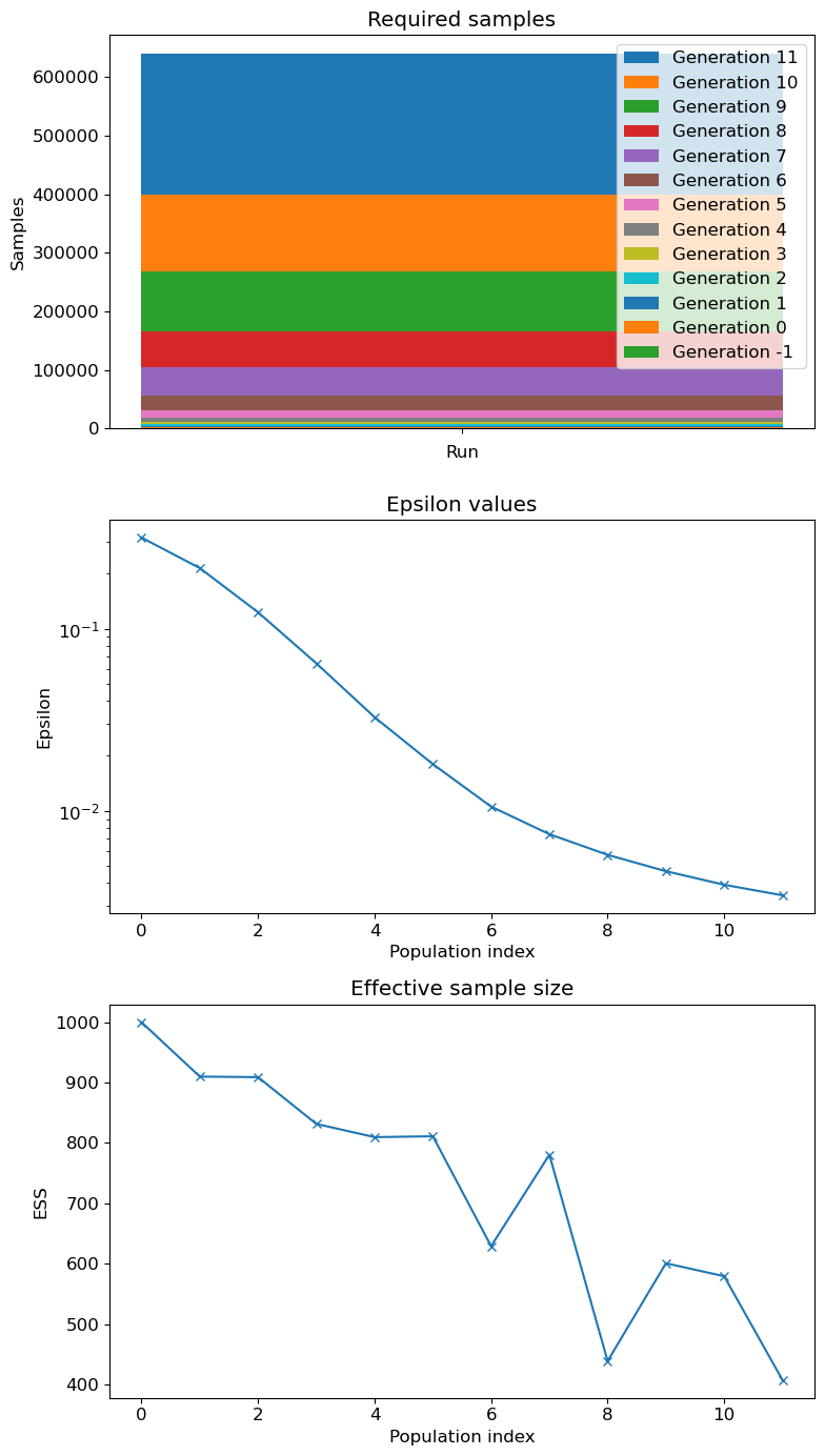
Figure 19 presents the posterior distributions for the heterogeneous configuration.
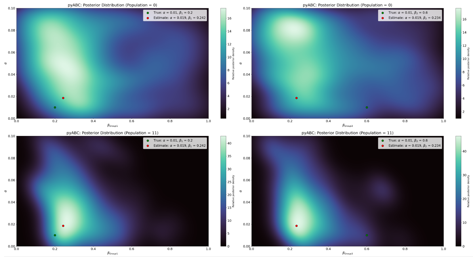
Figure 19a presents the posterior distribution of \(\alpha\) and \(\beta_{\text{Group1}}\). Unlike the homogeneous configuration, there is no observable linear relationship between the parameters. Instead, the pyABC iterative process reduces the parameter space and converges towards the pyABC estimate, which falls into the lightest hue of the high-density area. pyABC only slightly overestimates \(\alpha\) and \(\beta_{\text{Group1}}\), as the values are approximate in the second and first decimal points respectively. Although parameter estimation is successful and the true value sits on the cusp of the high-density area, there is evidence of a structural identifiability issue.
Similarly, Figure 19b presents the posterior distribution of \(\alpha\) and \(\beta_{\text{Group2}}\). There is some clear convergence around the pyABC estimates but the true values fall dramatically outside of the high-density area. Also, the distance between the true and estimated is considerably large. These findings indicate a structural identifiability issue. pyABC estimates of \(\beta_{\text{Group1}}\) and \(\beta_{\text{Group2}}\) are near approximates; it is possible that pyABC is unable to distinguish between the effects of two \(\beta\) parameters in the data, even though they are distinct. Thus, pyABC was unable to uniquely determine \(\beta_{\text{Group1}}\) from \(\beta_{\text{Group2}}\).
Appendix C: Robustness Checks
Additional analyses: Varying group proportions
This appendix presents the full derivation and supporting material for the group proportion analysis reported in Section 6. The aim was to investigate whether the proportion of agents allocated to each group influences infection dynamics in the heterogeneous configuration.
The total number of agents is decomposed into two groups:
| \[N = N_1 + N_2,\] | \[(7)\] |
where \(N_1\) and \(N_2\) denote the number of agents in Group 1 and Group 2, respectively. Each group was assigned its own infection parameter \(\beta\):
| \[N_1 = \beta_{\text{Group 1}} = 0.8957, \quad N_2 = \beta_{\text{Group 2}} = 0.0508.\] | \[(8)\] |
The population-weighted effective transmission rate can then be written as:
| \[\hat{\beta} = \theta_1 \beta_1 + (1 - \theta_1)\beta_2,\] | \[(9)\] |
where \(\theta_1 = N_1 / N \in [0,1]\) is the proportion of Group 1 agents in the population.
| Heterogeneous Config: ABM Parameters | |
|---|---|
| Parameter | Value |
| Number of Agents | 100 |
| Iterations (\(t\)) | 100 |
| Replications | 100 |
| Number of Agent Groups | 2 |
| \(\alpha\) | 0.1 |
| \(\beta_{\text{Group 1}}\) | 0.8957 |
| \(\beta_{\text{Group 2}}\) | 0.0508 |
| \(\gamma\) | 0.2 |
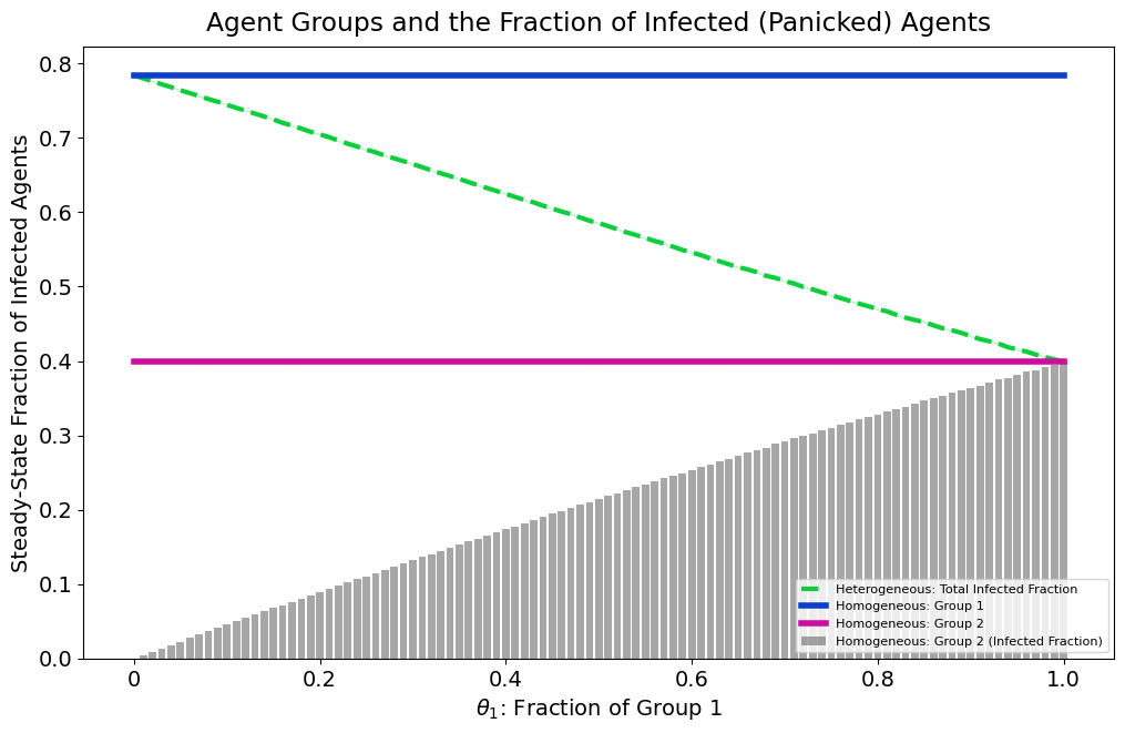
Heterogeneous \(\alpha\) parameters
This section contains the results of the pyABC exercise on the Heterogeneous Configuration of the case study ABM. Heterogeneity was expressed in \(\alpha\), rather than \(\beta\).
| pyABC ABC-SMC Algorithm Input | ||
|---|---|---|
| Parameter | Value | |
| Data | CDF (Number of Infected) | |
| Distance Function | RMSE | |
| Max. No of Populations | 12 | |
| Population Size | 1000 | |
| Epsilon (\(\epsilon\)) | Unspecified | |
| \(\beta\) | \(\mathcal{U}\) (0.0, 0.1) | |
| \(\alpha_{\text{Group1}}\) | \(\mathcal{U}\) (0.0, 1.0) | |
| \(\alpha_{\text{Group2}}\) | \(\mathcal{U}\) (0.0, 1.0) | |
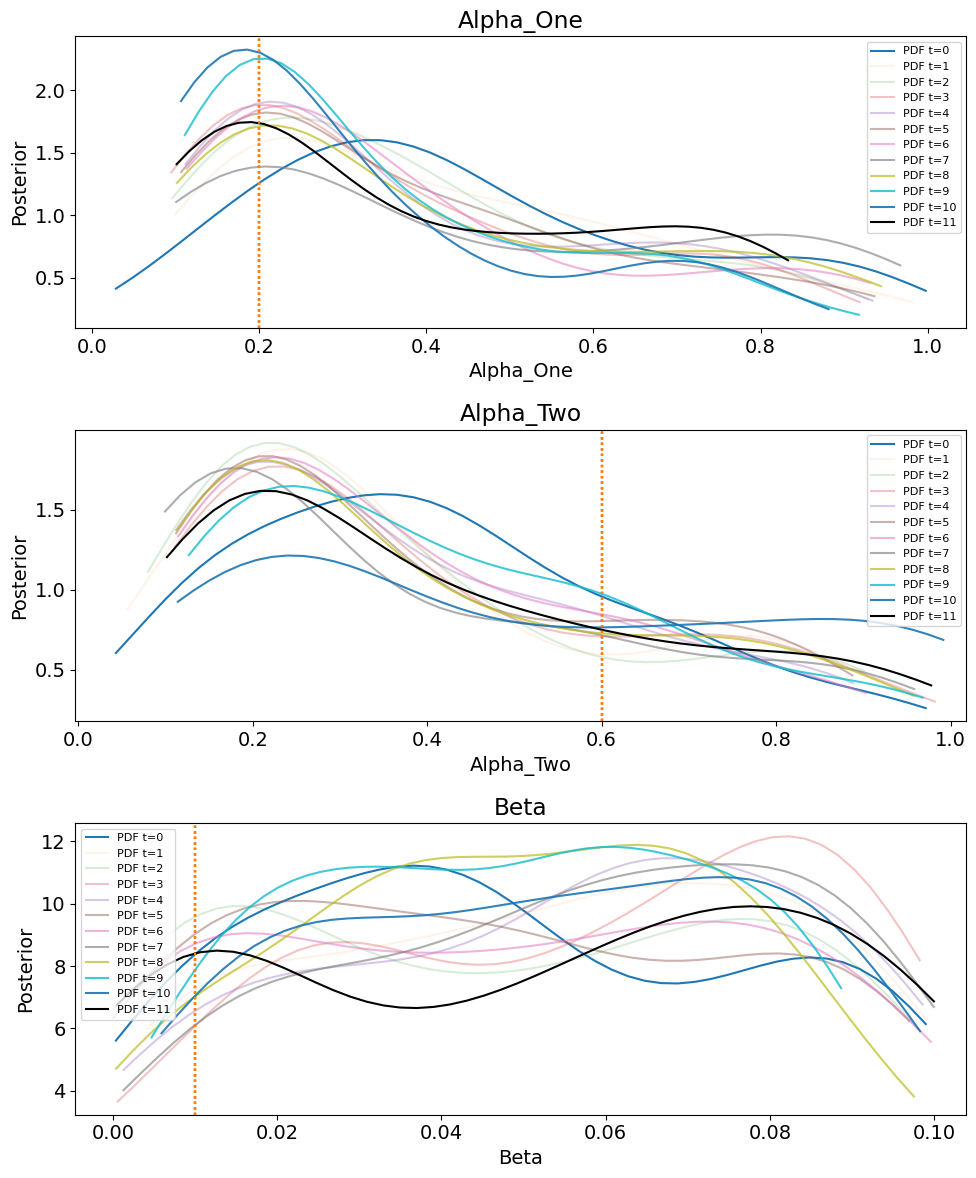
| Population | β | αGroup1 | αGroup2 |
|---|---|---|---|
| 0 | 0.0366 | 0.3253 | 0.3463 |
| 1 | 0.0699 | 0.2436 | 0.2433 |
| 2 | 0.0147 | 0.2321 | 0.2140 |
| 3 | 0.0823 | 0.1957 | 0.2359 |
| 4 | 0.0688 | 0.2126 | 0.2069 |
| 5 | 0.0218 | 0.2082 | 0.2230 |
| 6 | 0.0732 | 0.2302 | 0.2274 |
| 7 | 0.0738 | 0.2069 | 0.1871 |
| 8 | 0.0638 | 0.2049 | 0.2170 |
| 9 | 0.0613 | 0.2099 | 0.2470 |
| 10 | 0.0738 | 0.1856 | 0.2395 |
| 11 | 0.0776 | 0.1909 | 0.2090 |
Varying \(\beta\) parameters
This section presents the results of pyABC analysis on the Heterogeneous Configuration of the case study ABM, where the \(\beta\) parameters are numerically closer.
| Heterogeneous Config: ABM Parameters | |
|---|---|
| Parameter | Value |
| Number of Agents | 1000 |
| Number of Iterations (Time, \(t\)) | 1000 |
| Single Instance | 1\((t)\) |
| Number of Agent Groups | 2 |
| \(\alpha\) | 0.01 |
| \(\beta_{\text{Group1}}\) | 0.5 |
| \(\beta_{\text{Group2}}\) | 0.6 |
| \(\gamma\) | 0.1 |

| Population | α | βGroup1 | βGroup2 |
|---|---|---|---|
| 0 | 0.0113 | 0.1438 | 0.1426 |
| 1 | 0.0078 | 0.1427 | 0.1831 |
| 2 | 0.0126 | 0.1835 | 0.1834 |
| 3 | 0.0138 | 0.1632 | 0.1431 |
| 4 | 0.0125 | 0.1651 | 0.1422 |
| 5 | 0.0119 | 0.1646 | 0.3455 |
| 6 | 0.0116 | 0.4690 | 0.4075 |
| 7 | 0.0129 | 0.3867 | 0.4699 |
| 8 | 0.0114 | 0.3271 | 0.4714 |
| 9 | 0.0103 | 0.4079 | 0.7398 |
| 10 | 0.0106 | 0.3484 | 0.5724 |
| 11 | 0.0117 | 0.6321 | 0.2961 |
References
ALIFERIS, C., & Simon, G. (2024). Overfitting, underfitting and general model overconfidence and under-performance pitfalls and best practices in machine learning and AI. In G. J. Simon & C. Aliferis (Eds.), Artificial Intelligence and Machine Learning in Health Care and Medical Sciences (pp. 477–524). Springer International Publishing.
ANSTETT-COLLIN, F., Denis-Vidal, L., & Millérioux, G. (2020). A priori identifiability: An overview on definitions and approaches. Annual Reviews in Control, 50, 139–149.
AUGUSIAK, J., Van Den Brink, P. J., & Grimm, V. (2014). Merging validation and evaluation of ecological models to “evaludation”: A review of terminology and a practical approach. Ecological Modelling, 280, 117–128.
BANDARA, S., Schlöder, J. P., Eils, R., Bock, H. G., & Meyer, T. (2009). Optimal experimental design for parameter estimation of a cell signaling model. PLoS Computational Biology, 5(11), e1000558.
BANSAL, S., Grenfell, B. T., & Meyers, L. A. (2007). When individual behaviour matters: Homogeneous and network models in epidemiology. Journal of the Royal Society Interface, 4(16), 879–891.
BARREÑADA, L., Dhiman, P., Timmerman, D., Boulesteix, A.-L., & van Calster, B. (2024). Understanding overfitting in random forest for probability estimation: A visualization and simulation study. Diagnostic and Prognostic Research, 8(1), 14.
BAVEL, J. J. V., Baicker, K., Boggio, P. S., Capraro, V., Cichocka, A., Cikara, M., Crockett, M. J., Crum, A. J., Douglas, K. M., Druckman, J. N., Drury, J., Dube, O., Ellemers, N., Finkel, E. J., Fowler, J. H., Gelfand, M., Han, S., Haslam, S. A., Jetten, J., … Willer, R. (2020). Using social and behavioural science to support COVID-19 pandemic response. Nature Human Behaviour, 4(5), 460–471.
BEAUMONT, M. A. (2019). Approximate Bayesian Computation. Annual Review of Statistics and Its Application, 6(1), 379–403.
BEAUMONT, M. A. (2010). Approximate Bayesian computation in evolution and ecology. Annual Review of Ecology, Evolution, and Systematics, 41(1), 379–406.
BEAUMONT, M. A., Zhang, W., & Balding, D. J. (2002). Approximate Bayesian Computation in Population Genetics. Genetics, 162(4), 2025–2035.
BELLU, G., Saccomani, M. P., Audoly, S., & D’Angiò, L. (2007). DAISY: A new software tool to test global identifiability of biological and physiological systems. Computer Methods and Programs in Biomedicine, 88(1), 52–61.
BERESTYCKI, H., Desjardins, B., Weitz, J. S., & Oury, J.-M. (2023). Epidemic modeling with heterogeneity and social diffusion. Journal of Mathematical Biology, 86(4), 60.
BERNTON, E., Jacob, P. E., Gerber, M., & Robert, C. P. (2019). Approximate Bayesian computation with the Wasserstein Distance. Journal of the Royal Statistical Society Series B: Statistical Methodology, 81(2), 235–269.
BERRY, W. D., DeMeritt, J. H. R., & Esarey, J. (2016). Bias and overconfidence in parametric models of interactive processes. American Journal of Political Science, 60(2), 521–539.
BONABEAU, E. (2002). Agent-based modeling: Methods and techniques for simulating human systems. Proceedings of the National Academy of Sciences, 99(3), 7280–7287.
BUCHMANN, C. M., Grossmann, K., & Schwarz, N. (2016). How agent heterogeneity, model structure and input data determine the performance of an empirical ABM - A real-world case study on residential mobility. Environmental Modelling & Software, 75, 77–93.
CARRELLA, E. (2021). No Free Lunch when Estimating Simulation Parameters. Journal of Artificial Societies and Social Simulation, 24(2), 7.
CHATTOE-BROWN, E. (2023). Is agent-based modelling the future of prediction? International Journal of Social Research Methodology, 26(2), 143–155.
CHIS, O.-T., Banga, J. R., & Balsa-Canto, E. (2011). Structural identifiability of systems biology models: A critical comparison of methods. PLoS One, 6(11), e27755.
COOLEN, A., Sheikh, M., Mozeika, A., Aguirre-Lopez, F., & Antenucci, F. (2020). Replica analysis of overfitting in generalized linear models. arXiv preprint. Available at: https://arxiv.org/abs/2004.06329
CRANMER, K., Brehmer, J., & Louppe, G. (2020). The frontier of simulation-based inference. Proceedings of the National Academy of Sciences, 117(48), 30055–30062.
CSILLÉRY, K., Blum, M. G. B., Gaggiotti, O. E., & François, O. (2010). Approximate Bayesian Computation (ABC) in practice. Trends in Ecology & Evolution, 25(7), 410–418.
DEL Moral, P., Doucet, A., & Jasra, A. (2012). An adaptive sequential Monte Carlo method for approximate Bayesian computation. Statistics and Computing, 22, 1009–1020.
DEL Moral, P., Doucet, A., & Jasra, A. (2006). Sequential Monte Carlo samplers. Journal of the Royal Statistical Society: Series B (Statistical Methodology), 68(3), 411–436.
DI Molfetta, G. (2016). On the parameter identifiability problem in agent-based economical models. arXiv preprint. Available at: http://arxiv.org/abs/1602.01271
DONNAT, C., & Holmes, S. (2023). Modeling the heterogeneity in COVID-19’s reproductive number and its impact on predictive scenarios. Journal of Applied Statistics, 50(11-12), 2518–2546.
EDMONDS, B., Le Page, C., Bithell, M., Chattoe-Brown, E., Grimm, V., Meyer, R., Montañola-Sales, C., Ormerod, P., Root, H., & Squazzoni, F. (2019). Different modelling purposes. Journal of Artificial Societies and Social Simulation, 22(3), 6.
ELLISON, G. (2020). Implications of heterogeneous SIR models for analyses of COVID-19 (Nos. w27373; p. w27373). National Bureau of Economic Research.
ELSENBROICH, C., & Polhill, J. G. (2023). Agent-based modelling as a method for prediction in complex social systems. International Journal of Social Research Methodology, 26(2), 133–142.
FLORENS, J. P., & Simoni, A. (2021). Revisiting identification concepts in Bayesian analysis. Annals of Economics and Statistics, 144, 38.
FU, Y. X., & Li, W. H. (1997). Estimating the age of the common ancestor of a sample of DNA sequences. Molecular Biology and Evolution, 14(2), 195–199.
GAGLIARDI, R. (1967). Input selection for parameter identification in discrete systems. IEEE Transactions on Automatic Control, 12(5), 597–599.
GAO, F., Song, F., & Wang, J. (2013). Rational expectations equilibrium with uncertain proportion of informed traders. Journal of Financial Markets, 16(3), 387–413.
GODFREY, K. R., & Di Stefano, J. J. (1985). Identifiability of model parameter. IFAC Proceedings Volumes, 18(5), 89–114.
GRAZZINI, J., Richiardi, M. G., & Tsionas, M. (2017). Bayesian estimation of agent-based models. Journal of Economic Dynamics and Control, 77, 26–47.
GRIMM, V., & Railsback, S. F. (2005). Individual-Based Modeling and Ecology: Princeton, NJ: Princeton University Press.
GUILLAUME, J. H. A., Jakeman, J. D., Marsili-Libelli, S., Asher, M., Brunner, P., Croke, B., Hill, M. C., Jakeman, A. J., Keesman, K. J., Razavi, S., & Stigter, J. D. (2019). Introductory overview of identifiability analysis: A guide to evaluating whether you have the right type of data for your modeling purpose. Environmental Modelling & Software, 119, 418–432.
GULDEN, T. R., Hartnett, G. S., Vardavas, R., & Kravitz, D. (2021). Protecting the most vulnerable by vaccinating the most active. RAND Corporation.
GUSTAFSON, P., Gelfand, A. E., Sahu, S. K., Johnson, W. O., Hanson, T. E., Joseph, L., & Lee, J. (2005). On model expansion, model contraction, identifiability and prior Information: Two illustrative scenarios involving mismeasured variables [with Comments and Rejoinder]. Statistical Science, 20(2), 111–140.
GUSTAFSSON, L., & Sternad, M. (2010). Consistent micro, macro and state-based population modelling. Mathematical Biosciences, 225(2), 94–107.
HARTIG, F., Calabrese, J. M., Reineking, B., Wiegand, T., & Huth, A. (2011). Statistical inference for stochastic simulation models - Theory and application: Inference for stochastic simulation models. Ecology Letters, 14(8), 816–827.
HASSAN, S., Arroyo, J., Galán, J. M., Antunes, L., & Pavón, J. (2011). Asking the oracle: Introducing forecasting principles into agent-based modelling. Journal of Artificial Societies and Social Simulation, 16(3), 13.
HILL, A. L., Rand, D. G., Nowak, M. A., & Christakis, N. A. (2010). Emotions as infectious diseases in a large social network: The SISa model. Proceedings of the Royal Society B: Biological Sciences, 277(1701), 3827–3835.
IRANZO, V., & Pérez-González, S. (2021). Epidemiological models and COVID-19: A comparative view. History and Philosophy of the Life Sciences, 43(3), 104.
JIANG, B., Wu, T.-y., Zheng, C., & Wong, W. H. (2015). Learning summary statistic for Approximate Bayesian computation via deep neural network. arXiv preprint. Available at: https://arxiv.org/abs/1510.02175
JOUBERT, D., Stigter, J. D., & Molenaar, J. (2020). An efficient procedure to assist in the re-parametrization of structurally unidentifiable models. Mathematical Biosciences, 323, 108328.
KLINGER, E., & Hasenauer, J. (2017). A scheme for adaptive selection of population sizes in Approximate Bayesian computation - Sequential Monte Carlo. In J. Feret & H. Koeppl (Eds.), Computational Methods in Systems Biology (pp. 128–144). Springer International Publishing.
LIGMANN-ZIELINSKA, A., Kramer, D. B., Spence Cheruvelil, K., & Soranno, P. A. (2014). Using uncertainty and sensitivity analyses in socioecological agent-based models to improve their analytical performance and policy relevance. PLoS One, 9(10), e109779.
LJUNG, L., & Glad, T. (1994). On global identifiability for arbitrary model parametrizations. Automatica, 30(2), 265–276.
LU, J., Lin, A., Jiang, C., Zhang, A., & Yang, Z. (2021). Influence of transportation network on transmission heterogeneity of COVID-19 in China. Transportation Research Part C: Emerging Technologies, 129, 103231.
MARTÍNEZ, I., Wiegand, T., Camarero, J. J., Batllori, E., & Gutiérrez, E. (2011). Disentangling the formation of contrasting tree-line physiognomies combining model selection and Bayesian parameterization for simulation models. The American Naturalist, 177(5), E136–E152.
MAY, F., Giladi, I., Ristow, M., Ziv, Y., & Jeltsch, F. (2013). Metacommunity, mainland-island system or island communities? Assessing the regional dynamics of plant communities in a fragmented landscape. Ecography, 36(7), 842–853.
MCCULLOCH, J., Ge, J., Ward, J. A., Heppenstall, A., Polhill, J. G., & Malleson, N. (2022). Calibrating agent-based models using uncertainty quantification methods. Journal of Artificial Societies and Social Simulation, 25(2), 1.
MERKT, B., Timmer, J., & Kaschek, D. (2015). Higher-order Lie symmetries in identifiability and predictability analysis of dynamic models. Physical Review E, 92(1), 012920.
MOLLISON, D. (1995). Epidemic Models: Their Structure and Relation to Data. Cambridge: Cambridge University Press.
POHJANPALO, H. (1978). System identifiability based on the power series expansion of the solution. Mathematical Biosciences, 41(1-2), 21–33.
POLHILL, J. G., Hare, M., Bauermann, T., Anzola, D., Palmer, E., Salt, D., & Antosz, P. (2021). Using agent-based models for prediction in complex and wicked systems. Journal of Artificial Societies and Social Simulation, 24(3), 2.
PRITCHARD, J. K., Seielstad, M. T., Perez-Lezaun, A., & Feldman, M. W. (1999). Population growth of human Y chromosomes: A study of Y chromosome microsatellites. Molecular Biology and Evolution, 16(12), 1791–1798.
RAUE, A., Karlsson, J., Saccomani, M. P., Jirstrand, M., & Timmer, J. (2014). Comparison of approaches for parameter identifiability analysis of biological systems. Bioinformatics, 30(10), 1440–1448.
REEVES, D. C., Willems, N., Shastry, V., & Rai, V. (2022). Structural effects of agent heterogeneity in agent-based models: Lessons from the social spread of COVID-19. Journal of Artificial Societies and Social Simulation, 25(3), 3.
ROBERT, C. P., Cornuet, J.-M., Marin, J.-M., & Pillai, N. S. (2011). Lack of confidence in Approximate Bayesian computation model choice. Proceedings of the National Academy of Sciences, 108(37), 15112–15117.
ROTHENBERG, T. J. (1971). Identification in parametric models. Econometrica, 39(3), 577.
SACCOMANI, M. P., Audoly, S., & D’Angiò, L. (2003). Parameter identifiability of nonlinear systems: The role of initial conditions. Automatica, 39(4), 619–632.
SCHÄLTE, Y., Klinger, E., Alamoudi, E., & Hasenauer, J. (2022). pyABC: Efficient and robust easy-to-use approximate Bayesian computation. arXiv preprint. Available at: https://arxiv.org/abs/2203.13043
SHIN, M.-J., Guillaume, J. H. A., Croke, B. F. W., & Jakeman, A. J. (2015). A review of foundational methods for checking the structural identifiability of models: Results for rainfall-runoff. Journal of Hydrology, 520, 1–16.
SISSON, S. A., Fan, Y., & Tanaka, M. M. (2009). Correction for Sisson et al., Sequential Monte Carlo without likelihoods. Proceedings of the National Academy of Sciences, 106(39), 16889–16889.
SMAJGL, A., Bohensky, E., & Bohnet, I. (2007). Capturing heterogeneity in empirical agent-based models: A guideline. Fifth ESSA Conference in Social Simulation 2008, 6.
SOTTORIVA, A., & Tavaré, S. (2010). Integrating Approximate Bayesian computation with complex agent-based models for cancer research. In Y. Lechevallier & G. Saporta (Eds.), Proceedings of COMPSTAT’2010 (pp. 57–66). Heidelberg: Physica-Verlag HD.
STAN Development Team. (2025). Stan reference manual. Available at: https://mc-stan.org
SUN, Z., Fang, H., Di, L., & Yue, P. (2016). Realizing parameterless automatic classification of remote sensing imagery using ontology engineering and cyberinfrastructure techniques. Computers & Geosciences, 94, 56–67.
TALTS, S., Betancourt, M., Simpson, D., Vehtari, A., & Gelman, A. (2018). Validating Bayesian inference algorithms with Simulation-Based Calibration. arXiv preprint. Available at: https://arxiv.org/abs/1804.06788.
TAVARÉ, S., Balding, D. J., Griffiths, R. C., & Donnelly, P. (1997). Inferring coalescence times from DNA sequence data. Genetics, 145(2), 505–518.
THIELE, J. C., Kurth, W., & Grimm, V. (2014). Facilitating parameter estimation and sensitivity analysis of agent-based models: A cookbook using NetLogo and ’R’. Journal of Artificial Societies and Social Simulation, 17(3), 11.
THIEME, H. R. (1985). Local stability in epidemic models for heterogeneous populations. Mathematics in Biology and Medicine: Proceedings of an International Conference Held in Bari, Italy, July 18–22, 1983, 185–189.
THOMAS, L. J., Huang, P., Yin, F., Luo, X. I., Almquist, Z. W., Hipp, J. R., & Butts, C. T. (2020). Spatial heterogeneity can lead to substantial local variations in COVID-19 timing and severity. Proceedings of the National Academy of Sciences, 117(39), 24180–24187.
THURNER, S., Klimek, P., & Hanel, R. (2018). Introduction to the Theory of Complex Systems. Oxford: Oxford University Press.
TONI, T., Welch, D., Strelkowa, N., Ipsen, A., & Stumpf, M. P. H. (2009). Approximate Bayesian computation scheme for parameter inference and model selection in dynamical systems. Journal of the Royal Society Interface, 6(31), 187–202.
TURNER, B. M., & van Zandt, T. (2012). A tutorial on Approximate Bayesian computation. Journal of Mathematical Psychology, 56(2), 69–85.
VAN der Vaart, E., Beaumont, M. A., Johnston, A. S. A., & Sibly, R. M. (2015). Calibration and evaluation of individual-based models using Approximate Bayesian computation. Ecological Modelling, 312, 182–190.
VILLAVERDE, A. F., Evans, N. D., Chappell, M. J., & Banga, J. R. (2019). Input-dependent structural identifiability of nonlinear systems. IEEE Control Systems Letters, 3(2), 272–277.
WALLACE, R. B., & Ogawa, V. A. (Eds.). (2015). Assessing the Use of Agent-Based Models for Tobacco Regulation. Washington, D.C.: National Academies Press.
WALTER, E., & Lecourtier, Y. (1982). Global approaches to identifiability testing for linear and nonlinear state space models. Mathematics and Computers in Simulation, 24(6), 472–482.
WEISS, G., & von Haeseler, A. (1998). Inference of population history using a likelihood approach. Genetics, 149(3), 1539–1546.
WIELAND, F.-G., Hauber, A. L., Rosenblatt, M., Tönsing, C., & Timmer, J. (2021). On structural and practical identifiability. Current Opinion in Systems Biology, 25, 60–69.
WILLIAMS, B. K. (2011). Passive and active adaptive management: Approaches and an example. Journal of Environmental Management, 92(5), 1371–1378.
WINDRUM, P., Fagiolo, G., & Moneta, A. (2007). Empirical validation of agent-based models: Alternatives and prospects. Journal of Artificial Societies and Social Simulation, 10(2), 8.
XIE, Y. (2013). Population heterogeneity and causal inference. Proceedings of the National Academy of Sciences, 110(16), 6262–6268.
YATES, J. W. T., Evans, N. D., & Chappell, M. J. (2009). Structural identifiability analysis via symmetries of differential equations. Automatica, 45(11), 2585–2591.
ZBAIR, M., Qaffou, A., & Hilal, K. (2023). Approximate Bayesian estimation of parameters of an agent-based model in epidemiology. In S. Melliani & O. Castillo (Eds.), Recent Advances in Fuzzy Sets Theory, Fractional Calculus, Dynamic Systems and Optimization (Vol. 476, pp. 302–314). Springer International Publishing.