Party Competition with Costly Voting

University of Notre Dame, United States
Journal of Artificial
Societies and Social Simulation 29 (3) 4
<https://www.jasss.org/29/3/4.html>
DOI: 10.18564/jasss.6117
Received: 21-Dec-2024 Accepted: 04-Jun-2026 Published: 30-Jun-2026
Abstract
This study investigates political party competition within a two-dimensional policy space. It departs from existing computational models that typically assume full turnout. Specifically, it extends Laver and Sergenti’s (2012) ``baseline'' (chapter 5) framework by examining the impact of voting costs on six party system outcomes: voter turnout & citizen representation, mean party & winner eccentricity (i.e., polarization), and voter & abstainer profiles. Using agent-based simulations that vary the number of parties, voting costs, and party strategies (all-hunter, all-aggregator, and all-sticker party systems), the study finds that costly voting increases party eccentricity in small all-hunter systems, while reducing it in large all-hunter systems. It also finds that the ability of all-aggregator party systems to maximize citizen representation erodes with increases in voting costs. Across all types of party systems, it finds that abstainers arise at the extremes of the policy space, and grow more moderate as costs rise. Theoretically and methodologically, the research uses experiments in a computational setting, and applies fractional polynomial regression to analyze the effect sizes of the inputs on the outcomes. The models, which integrate classic spatial models of party competition with the ``calculus of voting model,'' yield results which reveal complex interdependence between voting behavior, party behavior, and system-level properties.Introduction
Spatial models of party competition often assume full turnout. In his canonical work, Downs described this assumption as simultaneously useful and false: “We have assumed that voting is a costless act, but this assumption is self-contradictory because every act takes time. In fact, time is the principal cost of voting: time to register, to discover what parties are running, to deliberate, to go to the polls, and to mark the ballot. Since time is a scarce resource, voting is inherently costly” (1957 p. 265). This study loosens the costless voting assumption in order to examine how voting costs shape political participation, party behavior, citizen representation, and other properties of party competition.
Party competition with costly voting is a computational model that adds voting costs to Laver and Sergenti’s baseline model of party competition (2012 Chapter 5) (hereafter, L&S), which is itself an extension of earlier formal and computational spatial models of party competition. The seminal work on party competition in the formal spatial tradition takes place in a one-dimensional policy space, with two parties, and citizens distributed normally around the center of that space (Downs 1957). Beyond this basic setup, scholars have long sought to examine a wider range of scenarios—more policy dimensions, more parties using more varied party strategies, more diverse distributions of citizens with more varied motivations and capabilities—in order to expand the range and verisimilitude of the model. This expanded range of questions does not usually allow for analytically tractable solutions using formal mathematical approaches, and so, beginning with Kollman et al. (1992), scholars have built computational simulations of party competition (de Marchi 1999; Kollman et al. 1998; Laver 2005; Muis 2010; Reinermann 2014; Schumacher & Vis 2012; Wright & Sengupta 2015).
These models embody the features of complexity science, which distinguishes between agents in the policy space on the input side, and aggregate features of the political system on the outcome side. Politics is conceptualized as a dynamic and interdependent process, with individual citizens and parties adapting to each other and the environment. For example, a citizen’s decision to shift from voting to abstaining can set in motion a cascade of reactions that touches all actors of the system in subsequent rounds. This process yields emergent and often non-obvious adaptations and outcomes, which arise without the intention or design of the actors in the system.
The main contribution of party competition with costly voting is to endow citizens with the capability of deciding whether to vote or abstain. Some prior work treats abstention. Fowler & Smirnov (2005) and Kernell & Lamberson (2023) publish computational models with variable turnout, but the turnout decision is a function of social factors rather than voting costs. Also, in Bendor et al. (2003), citizens face costs and are adaptive with respect to turnout, but parties are not adaptive.1
The model examines six system-level outcomes—voter turnout & citizen representation, mean party & winner eccentricity (i.e., polarization), and voter & abstainer profiles—to understand the effect of voting costs. Apart from costly voting, I leave many of the other assumptions from Chapter 5 of L&S in place so that knowledge accumulates from that baseline, and is comparable to other related models (Jackson 2003; De Marchi 2003).
Under full turnout, citizens face a relatively simple task: identify the nearest party and vote for it. By contrast, a variable turnout model requires that we endow citizens with the ability to evaluate not only the policy locations of other parties, but also the electoral strength of parties, and compare the utility derived from these factors against voting costs. If policy-based utility exceeds cost, they vote; otherwise, they abstain.
In the models here, parties are one of three types, following L&S: “hunters” are insatiable vote-seekers who take a small policy step each time step, seeking to increase their vote share; “aggregators” seek to be good representatives by adapting towards the mean policy location of their voters; and “stickers” are principled policy adherents, who never adapt from their policy position at birth. These heuristics are formalized below.
L&S establish a set of baseline models (in chapter five) in which each party strategy competes with other parties of the same strategy—all-hunter, all-aggregator, and all-sticker party competition. Theoretically, two of these scenarios have deep intrinsic importance. The all-hunter models adopt a common assumption about party behavior within the long spatial tradition of party competition. One high-level result in L&S shows that two vote-hunters competing in a two-dimensional policy space converge to within about \(0.19\sigma\) of the median voter, replicating in spirit (though not by formal theorem) the centripetal result of the one-dimensional Median Voter Theorem. They further show that adding more hunters increases the average policy divergence of the parties from the median. In this paper, we examine whether and how parties and citizens adapt relative to these baseline results in the face of costly voting.
The all-aggregator models are interesting for a different and more novel reason. As a matter of politics, the aggregator orientation is normatively attractive; however, it lacks the deep disciplinary foundations of the vote-seeking assumption. Nevertheless, L&S link all-aggregator competition to a long tradition of discoveries with roots in geometry, with applications in fields that include electrical engineering (image and audio compression), ecology (the distribution of animal nests), urban planning (the allocation of resources such as fire stations), wireless sensor network deployment, and electoral redistricting where early computational approaches (Hess et al. 1965) minimized the summed squared distance from each citizen to a district center.
The general challenge across these domains is to find an efficient way to distribute a given set of points within a landscape of interest. In politics, when a collection of aggregators is operating, they will maximize the representativeness of a party system. Indeed, L&S show that the aggregator algorithm is equivalent to “Lloyd’s Algorithm,” developed by Stuart Lloyd in 1957 at Bell Labs (Lloyd 1982) to compress signals efficiently with minimum error. Lloyd’s algorithm is also the foundation of \(k\)-means clustering—arguably the most widely deployed algorithm in modern data science and machine learning (Hartigan & Wong 1979; MacQueen 1967). The equivalence between all-aggregator party competition and k-means clustering means that every all-aggregator configuration is, formally, a k-means partition of the citizen distribution into k support clusters, each centered on a party’s policy position. I formalize the algorithms and outcomes later; for now, it is enough to note that the all-aggregator system instantiates a principle of optimal spatial partitioning that recurs across the physical, natural, and social worlds. When voting costs are low, all-aggregator competition produces highly symmetric distributions of parties and voter support. Here I explore whether and how costly voting erodes this result.
The results here replicate the baseline full-turnout findings from L&S and add three main insights about the dynamics of party competition with costly voting. First, in party systems consisting of all-hunters, voting costs interact with the number of parties in an unexpected way: costs increase party eccentricity in small party systems, while reducing it in large party systems. Because representation is closely tied to party eccentricity, the inverse holds for citizen misery, which declines as costs rise in small party systems but increases in large ones.
Second, in all-aggregator competition—where the central advantage of the strategy is that it delivers optimal representation for a given number of parties—costly voting reveals the vulnerability of this outcome: as voting costs rise, the propensity of the algorithm to maximize representation breaks down.
Third, in party systems of all types, abstention begins at the extremes of the policy space and spreads inward as costs rise, providing theoretical support for the primacy of “abstention due to alienation” over “abstention due to indifference” (Brody & Page 1973).
In the next section, I develop the model of party competition with costly voting, describe the policy and time dimensions of the model, and detail the political actors and their competencies. I also define the six system-level outcomes. Then, I report the results in two subsections—one each for all-hunter competition and all-aggregator competition. Last, I discuss the results and conclude. The first appendix reports the replication of L&S chapter 5 no-cost results as the baseline of comparison. Subsequent appendices report the less interesting results of the all-sticker models and the effective number of parties outcome.
A Model of Party Competition with Costly Voting
The policy space and time
Party competition is represented as taking place within a Cartesian coordinate system, \(\Phi\). Following L&S, I use two dimensions, \(X\) and \(Y\), which can represent two conceptually continuous independent policy dimensions.
| \[\Phi = X \times Y\] | \[(1)\] |
For example, the horizontal \(X\) axis can represent an economic left/right continuum of policy positions, while the vertical \(Y\) axis may represent a distribution of socially liberal/conservative policy positions. For the purposes of the agent-based model, the space is operationalized as a discrete, finite grid of \(71 \times 71\) integer coordinates, ranging from \([-35, 35]\) on both the X-axis and Y-axis. This results in 5,041 discrete policy locations \((x, y) \in \Phi\), where \(x, y \in \{-35, -34, \dots, 34, 35\}\). The origin \((0,0)\) represents a centrist location on both dimensions.
Empirical studies of politics generally support a low-dimensional specification of a policy space, though of course there is a great deal of national variation. The economic and social dimensions are especially well-founded (Bakker et al. 2012; Benoit & Laver 2006). A two dimensional assumption is also commonly embodied in national election studies. For example, the British Election Study includes two survey modules of six questions each to place citizens on the economic left/right and social liberal/conservative dimensions (Fieldhouse et al. 2024).
The model advances in discrete time: All actors make their moves (described below) simultaneously at each tick of the clock. A tick can be thought of as an election cycle, or as an opinion polling cycle.
Citizen actors
Citizens are one of the two main actors in the simulation. The model includes 1,000 citizen agents, \(i \in \{1, \dots, 1000\}\). Each citizen \(i\) is endowed with a fixed policy preference \(\mathbf{p}_i = (x_i, y_i)\), representing their most-preferred policy position in the space \(\Phi\). These preferences remain constant throughout the simulation.
The initial location of the 1,000 citizen agents in the policy space is determined by a continuous, two-dimensional Normal distribution, \(Z(x, y)\), centered at the origin \((0, 0)\) with a standard deviation of \(\sigma=10\) policy units for both dimensions. The distribution is defined by the probability density function:
| \[Z(x, y) = 1000 \cdot \frac{1}{2\pi \cdot 10^2} e^{-\left( \frac{x^2}{2 \cdot 10^2} + \frac{y^2}{2 \cdot 10^2} \right)}\] | \[(2)\] |
While the theoretical distribution is continuous, the agents are sampled from this continuous distribution and their fixed preferences \(\mathbf{p}_i\) are then assigned to the nearest discrete policy location within the grid \(\Phi\) defined in Section 2.1. This method ensures that the population density reflects the theoretical continuous distribution, while still accommodating the discrete nature of the ABM’s grid-based implementation.
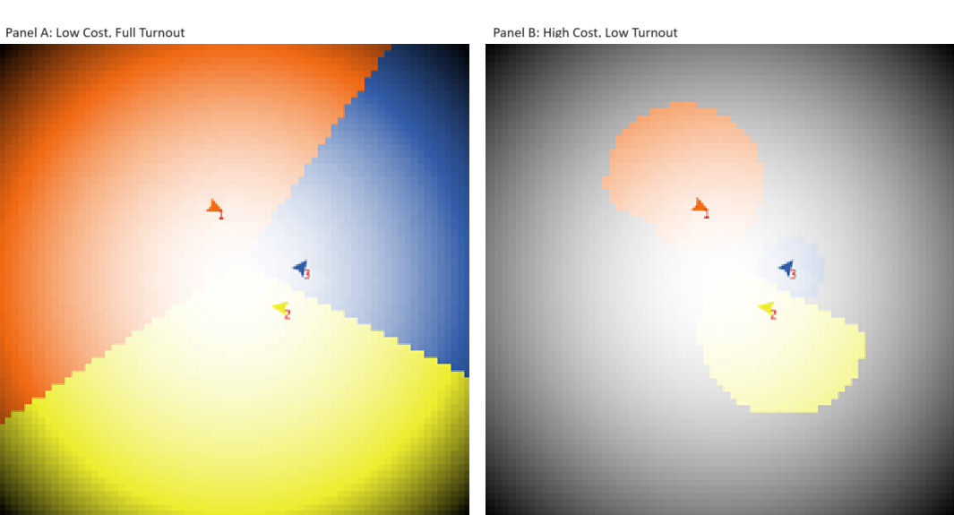
Foreshadowing Figure 1 below, in the interface of the computational model, the citizens are rendered visually as a gradient of colored sites in the policy space, with population density ranging from bright (high density) to black (low density). That is, the higher density sites at or near \((0, 0)\) are brighter and the low density extreme positions are blacker. Since the interface is in 2D, the citizens appear as if looking down at the top of a bell. In the images presented here, the site densities are log-transformed so that the color gradient’s transition to black is more gradual.
Two features of the citizen distribution will serve as reference points for results that arise from the model. First, the median policy position of citizens is \((0, 0)\). This location is a valuable reference point because it represents the equilibrium outcome of the Median Voter Theorem under full turnout in all-hunter competition. Second, in a bivariate normal distribution, the mean policy distance of the citizenry from the median citizen is \(12.5\) policy units, or \(1.25\sigma\).
Citizens are adaptive with respect to their turnout decision; however, I retain the assumption that the population holds fixed policy positions in order to compare my results to the L&S baseline. This isolation strategy—loosening one assumption at a time while holding others constant—is central to the cumulative research program in this tradition (Laver & Sergenti 2012 Chapter 3). It is important nonetheless to note that citizens in the real world are known to adapt their policy preferences, and that this adaptation can generate distributions that are skewed, multimodal, or otherwise asymmetric. Computational treatments of adaptive citizen attitudes have a rich and largely separate tradition in the opinion-dynamics literature (Lorenz et al. 2021; Troitzsch 2021), and work integrating that tradition with spatial models of party competition is now emerging (Geyer & Mellacher 2025). Within the spatial tradition itself, L&S parameterize the citizen distribution by allowing for multiple subpopulations with variable means and variances; future contributions to this program will plausibly combine those distributional generalizations with the costly-voting capabilities developed here, with adaptive citizen attitudes, and with empirical calibration to specific party systems (Laver 2005; Laver & Sergenti 2012 Chapter 11).
Party actors
The second type of actor is the political party. A set of two to ten parties \(P\) occupy the policy space such that the number of parties is \(P = \{p_1, p_2,\dots, p_j\}\), where \(2\leq j\leq 10\).
Each party seeks votes following one of three different strategies, set exogenously at startup and held constant. At any given time, each party \(p_j\) occupies a location in the policy space and updates their policy location over time according to their strategy. Party location and movement is measured on a continuous scale.
Parties here are not rational actors with full information; instead, they are boundedly rational and use “informal rules of thumb” to govern their policy-taking decisions (Laver & Sergenti 2012 p.28). They are adaptive and adopt one of three strategies defined using algorithms from L&S. Each rule corresponds to a different ideal-type party goal: “hunters” seek votes, “aggregators” seek to be good representatives of their voters, and “stickers” are principled position takers. Scholars seeking to expand upon the set of strategies have examined the performance of other rules.2
Hunters are vote-maximizers who conform to the standard party strategy in the spatial tradition. The seminal computational work on adaptive party competition was conducted by Kollman et al. (1992, 1998), who described parties as “adaptive organizations competing for votes in a multi-dimensional issue space” that respond to past levels of electoral support by “incrementally adapting their platforms” (Kollman et al. 1998 p.141). Their specific algorithm, however, requires parties to sample multiple counterfactual policy positions each cycle and adopt the best—a relatively information-rich heuristic. L&S’s hunter rule is information-poor by comparison: a party knows only whether its last move increased or decreased support and adopts a “win-stay, lose-shift” learning rule (Nowak & Sigmund 1993). This structure places it in a lineage of adaptive learning algorithms with broad cross-disciplinary currency: it is a foundational rule in evolutionary game theory, an empirical pattern in animal foraging, a simple instance of model-free reinforcement learning, and a precedent in adaptive models of voter behavior (Bendor et al. 2003). The Hunter rule is therefore a behaviorally and biologically plausible learning rule.
Operationally, L&S’s hunters take a one-unit policy step at each time increment. The direction of their step varies depending on their electoral performance in the previous round. As long as their last step yields an increase in vote share, they take another step in the same direction; however, if they experience a loss of vote share, they try a step in a different direction, randomly turning between 90 and 270 degrees from their current heading. Hunters adapt slowly in the short run because they take small steps, but in the long run they are opportunistic with respect to policy and willing to travel anywhere for votes. They neither perceive nor respond to the locations of other parties or the policy preferences of citizens; even so, the hunter is indirectly influenced by both, because these factors shape citizen behavior.
Aggregators are good representatives. At each time step they adopt the mean ideal point of their voters in the last election. They are not attentive to, nor directly responding to, other parties, the policy preferences of non-voting supporters, and non-supporters.
Stickers are policy-oriented parties who do not adapt. They value policy integrity over representativeness and electoral success. They are neither aware of, nor responsive to, anything in the party system. They adopt a policy location at startup, and never move.
Measuring distance
Policy distance \(d\) between two locations in the policy space is a building block of several outcomes. It is measured here as the square root of the sum of the squared differences of each coordinate. Following L&S, I convert all distance measures from policy units to the scale of the \(\sigma\) of the citizen population (here, 10 policy units). This transformation provides a convenient scale free metric, and makes the results easily comparable to the baseline full turnout models in L&S (as well as any other set of results based upon a normally distributed citizen population). Suppose there are two sites \(s_i\) and \(s_j\) with positions \((x_i, y_i)\) and \((x_j, y_j)\). The distance between them is
| \[d(s_i, s_j)=\frac{\sqrt{(x_i - x_j)^2 + (y_i - y_j)^2}}{\sigma}\] | \[(3)\] |
Citizen party preferences and turnout utility
Returning to citizens, I now define their party preferences and turnout decision. In order to so, I adopt a set of standard assumptions of the spatial modeling tradition. First, citizens have perfect information about each party’s current policy location. Second, their preferences over policies are single-peaked and declining monotonically with distance from their own policy location. Thus, they always prefer the closest party.3 Their preferences follow a quadratic loss function that declines with the distance from their own location. Thus, utility is at a maximum of zero at their own location, and declining as the square of the distance to any other policy location (Adams et al. 2005).
Each citizen calculates a utility \(U_i\) for participating in the election. The utility function here builds upon the calculus of voting model, with origins in Hotelling (1929) and Downs (1957). The formal rendering of the calculus of voting was first introduced by Riker & Ordeshook (1968), who expressed turnout utility as a function of a) policy benefit; b) the probability of casting the decisive vote; c) the cost of voting; and d) the duty a citizen feels towards the act of voting. Here, I simplify by considering only the policy benefit and the cost of voting, where the utility for a citizen \(z_i\) of participating in an election is a function of their individual policy-based benefit, \(B_i\), and the cost of voting \(C\)
| \[U_i=B_i-C\] | \[(4)\] |
Here, the cost of voting \(C\) is assumed to be equal for all citizens, and takes negative values to mirror the benefit term, \(B_i\), which takes negative values. Low costs are large negative values and higher costs approach zero from below. Voting costs in the model vary as \(C \in \{-900, -700, -500, -300, -100\}\). These values are selected to generate a realistic range of turnout.4 The highest cost, \(C=-100\), is selected because it always generates at least some turnout; when costs are set to \(-100\), only citizens relatively near to a party will have a policy benefit greater than the cost.
The policy-based benefit parameter \(B_i\) is a function of the location of multiple parties in the policy space. At each time step, a citizen will examine the menu of party policy options, and draw motivation to participate as a function of a) potential policy gains from their preferred party’s success, and b) threats from success by alternative parties. I follow Chen (2011) who proposes a utility function for multi-party political competition with variable turnout. He decomposes \(B_i\) into two components: The policy benefit \(F_i\) from the citizen’s most “favored” party \(p_{f,i}\) at location \((x_{f,i}, y_{f,i})\); and the benefit \(H_i\) derived from the policy threat from the citizen’s most “hated” party \(p_{h,i}\) at location \((x_{h,i}, y_{h,i})\)
| \[B_i=F_i + H_i\] | \[(5)\] |
Each citizen identifies their most favored and hated parties using a function that identifies the parties at the minimum and maximum distances from a list that includes the distances to all parties. The vote shares of \(p_{f,i}\) and \(p_{h,i}\) are \(e_f\) and \(e_h\), respectively.
With these, we define \(F_i\) and \(H_i\). For a given citizen \(z_i\), the utility derived from their most favored party is a function that increases with its electoral strength \(e_f\) and declines with its relative distance
| \[F_i=-\left(\frac{d(z_i, p_{f,i})}{e_f}\right)\] | \[(6)\] |
The utility derived from their most hated party is an increasing function of its strength \(e_h\) and relative distance
| \[H_i={e_h} d(z_i, p_{h,i})\] | \[(7)\] |
Thus, \(F_i\) is declining as a negative quadratic loss function, while \(H_i\) is increasing quadratically as the distance to those parties increases. Both terms are weighted by the electoral strength of the parties to reflect the fact that a citizen derives a larger motivation from strong parties (i.e., a larger potential gain by a strong preferred party and a larger potential threat by a strong hated party). For the most-favored party, the weighting factor inflates the utility as the inverse of the vote share. For the hated parties, it does so as a multiple of the vote share.
In sum, citizens are endowed with the following capabilities: a) they identify a most-preferred party and a most-hated party; b) they evaluate the utility associated with the location and electoral support of these parties in the policy space; and c) they make a binary decision about whether to vote for their preferred party or abstain by evaluating \(U_i\).
Voters and abstainers
Having defined citizens \(Z\) and the utility for voting \(U_i\), we can define two subsets of citizens, voters \(Z_V\) and abstainers \(Z_A\). Voters derive benefits that exceed costs, and abstainers face costs that exceed benefits.
| \[\begin{aligned} Z_V = \{ z_i \in Z \mid U(z_i) > 0 \} \\ Z_A = \{ z_i \in Z \mid U(z_i) \leq 0 \} \end{aligned}\] | \[(8)\] |
Representative screenshots of the model interface are rendered in Figure 1 for the case of three parties competing under low and high voting costs in panels A and B, respectively. Parties are represented as colored and numbered arrows, and citizens are represented as the colored patches with voters matching the color of their nearest party and abstainers on a grayscale. In Panel A, where voting costs are set to be very low, citizens throughout the policy space are voting. In Panel B, where voting costs are high, each party enjoys a relatively small island of voter support while citizens through most of the space are abstaining (including at the center).
Outcomes
I examine six party system outcomes in the main paper. Two come from L&S: party eccentricity and citizen misery. I follow their approach to conceptualization and measurement. In Appendix C, I also measure and report party system fragmentation, which is included in L&S. Four outcomes are new because their relevance only arises in the face of costly voting: turnout, winner eccentricity, and voter & abstainer eccentricity.
Turnout
Citizen turnout captures the degree of political participation and is measured as \(T\), the percentage of citizens who vote in each election. Let the percentage of \(Z_V\) in \(Z\) be calculated as:
| \[T=\frac{|Z_V|_{\text{card}}}{|Z|_{\text{card}}}\cdot 100\] | \[(9)\] |
Citizen representation
Citizen representation taps into the policy congruence between parties and the citizenry. How well do the positions of the parties correspond with the preferences of the citizens? Representation is measured using misery \(M\) which is the mean distance between the location of each citizen’s ideal point and the policy position of their most favored party. Misery increases as the mean distance of the nearest party increases. It is computed as
| \[M = \frac{1}{|Z|_{\text{card}}} \sum_{z=1}^{i} d(z_i, p_{f,i})\] | \[(10)\] |
A minimum of \(M=0\) will arise when a different party occupies each citizen’s ideal point. Of course, we will not examine party systems with so many parties, and so it is only a theoretical baseline for comparison.
A more interesting reference point for misery arises from the science of other fields, which has shown that representation can be optimized. As described above in Section 1.10, L&S show that the aggregator algorithm (when competing within a system of other aggregators) is known to find this optimal level of representation. Critically, this optimal system-level representativeness is an emergent property: no individual aggregator is trying to maximize system representativeness; each is doing only local optimization—adapting to its own current supporters—and yet the collective configuration achieves a global optimum (Laver & Sergenti 2012 p. 99). This emergence-from-local-rules property is the substantive heart of the all-aggregator result and the reason it generalizes to so many other domains.
Specifically, given a set of parties \(P\), an all-aggregator system minimizes \(M\) at a configuration that L&S identify as a centroidal Voronoi tessellation (CVT): a highly regular geometric pattern in which the electorate is partitioned into compact voting blocks centered on party positions. Three additional properties of this configuration are worth noting. First, Lloyd’s algorithm finds a local rather than a global minimum, so the algorithm need not converge to the same configuration from every starting point. Second, because the underlying citizen distribution is rotationally symmetric, the exact locations of parties vary across runs even when the system’s geometric structure does not (a given number of parties will align at different points along the circumference of a circle with a fixed radius). Third, as the number of parties grows, the system passes through a phase transition in the formal sense: a qualitative reorganization of the system’s macrostate as a control parameter (here, the number of parties) crosses a critical value. Around five parties, the hollow configuration—with all parties on a circumference and an empty center—ceases to be \(M\)-minimizing. Beyond this threshold, the optimal arrangement is centrally occupied, with one party at the center surrounded by others on a circle. Near the transition, both configurations yield similar \(M\) and Lloyd’s algorithm may converge to either depending on initial conditions. Computational geometers (Du et al. 1999) refer to these two regimes as (a) hollow and (b) centrally-occupied configurations. The transition is the reason all-aggregator dynamics produce qualitatively different outcomes in small versus large party systems. Together, these properties imply that the final configuration depends on the random starting locations of parties, which I discuss below.
Party eccentricity
Party eccentricity is a concept defined as the policy divergence of the parties in the system relative to the median citizen. When party eccentricity is low, the party system is populated with parties that compete near the median citizen’s ideal point, and when it is high, they compete far from their ideal point. This concept is sometimes referred to as “party polarization” in the political behavior tradition, though I avoid the term because in other uses it also evokes a form of extraordinary conflict that is categorically distinct from mere policy-difference (Schedler 2023). Here, party eccentricity \(E\) is measured as the average of the proximity between each party \(p_j\) and the citizen median location \((0,0)\) using the distance metric described above
| \[E = \frac{1}{|P|} \sum_{p=1}^{j} d(p_j, (0,0))\] | \[(11)\] |
Values of \(E\) can be compared with the reference values of the citizen distribution, \(0\) and \(1.25\sigma\), defined above in Section 2.8.
Winner eccentricity
Winner eccentricity is like party eccentricity, but with a focus on the winning platform rather than the mean of all party platforms: it defines the policy divergence between the winning party and the median citizen. When low, the winner competes relatively near the median citizen’s ideal point, and when high, it competes relatively far from their ideal point. Winner eccentricity \(W\) is measured as the distance between the platform of the winning party \(p_w\) and the median citizen location \((0, 0)\) using the distance metric described above
| \[W = d(p_w, (0,0))\] | \[(12)\] |
As with the measure of party eccentricity, a value of \(W=0\sigma\) will indicate that the winning platform is at the location of the median citizen, and a value of \(W=1.25\sigma\) will indicate that it is competing at the same distance from the median citizen as the mean of the citizen distance from the median citizen.
Citizen eccentricity
Citizen eccentricity captures the relative location of each citizen vis-à-vis the location of the median citizen. As discussed above, mean citizen eccentricity is 1.25\(\sigma\) for the population as defined here. It is invariant because the models here hold the citizen distribution constant. However, the mean eccentricity of voting and abstaining subsets will vary. In particular, mean eccentricity of abstainers \(E_{Z_a}\) will summarize the divergence of abstainers from the median citizen. Abstainer eccentricity is defined as
| \[E_{Z_a} = \frac{1}{|Z_a|_{\text{card}}} \sum_{z_a=1}^{i} d\left(Z_{a_i}, (0,0)\right)\] | \[(13)\] |
Research Design
Here I describe the model's initialization and run-time procedures. Then, I describe the experimental design.
Initialization and process overview
At initialization, the following are scheduled in order. First, a new random seed is established and values for the number of parties and voting costs are set. Then, citizens are distributed in the policy space. Next, parties are distributed with a location drawn randomly from the same Normal distribution used to place the citizenry. They are assigned their strategy, a random heading, and an equal share of the vote. Finally, citizens examine the initial distribution of the parties and decide whether to vote or abstain, and party vote shares are calculated.
At each time step, the following are scheduled in order. First, parties adapt their policy location following their strategy, synchronously. Then, citizens examine the new location of the parties in the policy space, compute their utility for voting, and either vote for the nearest party or abstain. Citizens also act synchronously. Finally, election results and performance outcomes are calculated, and the process repeats. The only process with a random component is the hunter rule, which includes policy adaptation using a random heading as described above.
The model is implemented using NetLogo v.6.2.2 (Wilensky 1999) and available here: https://www.comses.net/codebase-release/371ce1bf-2403-4435-a53f-292365b4e32c/. Documentation includes a model description following the ODD protocol (Grimm et al. 2010).
The experiments
The computational experiments follow the design used in chapter five of L&S, with small modifications. L&S conduct experiments under three scenarios: one for competition among hunters; a second for competition among aggregators, and a third for competition among stickers.
Like them, I vary the number of political parties in each experiment between two and ten. At baseline under full turnout, I set the cost of voting arbitrarily low — at -10,000 — in order to approximate full turnout conditions. Those baseline results are reported in Appendix A. Beyond this, I also vary the cost of voting across five values, which generate realistic variation in turnout. Taken together, the parameter space for each scenario reported here in the main paper includes nine settings for the number of political parties and five cost settings, for a total of 45 unique combinations.
The goal of this research is to estimate the mean of each outcome across this parameter space for each scenario. The experimental designs are established in terms of four features of the simulations. The first three follow the norms and reasoning detailed in L&S. First, for each experiment I distinguish between runs, repetitions, and iterations. A run corresponds with a single location in the parameter space. Each run may be repeated several times depending upon whether the process is ergodic or not (described below). A repetition will hold the experimental variables constant, but start from a different random seed. Finally, each repetition iterates through the schedule described above some finite number of times, producing values for the set of outcomes at each iteration.
Second, I distinguish between a transition state and a steady state. A given repetition of the model is said to be in a steady state when the expected value of the outcome for each iteration is constant over time. None of these runs initialize in steady state. Instead, initial iterations are sensitive to the random components of the startup values of each repetition. A given repetition moves through a transition state before arriving at a steady state. Even the sticker model, which for L&S is in steady state at initialization, transitions under costly voting because it requires some number of iterations to allow for citizens to adjust their turnout decisions to the turnout decisions of the other citizens. The initial iterations of the transition state are discarded as model burn-in.
Third, I distinguish between the type of temporal process operating within each of the three experiments. All-hunter party competition generates a stationary and ergodic process of the outcomes; that is, beyond the initial iterations, it tends towards a single distribution of the outcome, regardless of the initial conditions. In this circumstance, and after discarding the initial iterations as burn-in, the experimental design can rely upon a time average of the outcomes over some set of steady state iterations from a single repetition. For the other two scenarios — all-sticker and all-aggregator — the process of party competition is stationary, but not ergodic; that is, the steady state outcome of a given repetition depends in part on the initial conditions. Specifically, it depends upon the random location of the parties at birth. Thus, I collect data about the outcomes across a range of initial conditions using the last iteration from a large number of repetitions. With these, I compute an ensemble average of the outcomes.
Fourth and finally, note that aggregate-level stability (i.e., steady state) does not imply stability at the level of individual actors. A variety of micro-level behaviors can give rise to a steady state. In particular, steady state in our models takes the form of “settling” behavior in the all-aggregator context and “orbiting” behavior in the all-hunter context. Aggregators settle, which is to say that each converges to a specific point (a “point attractor”) in the policy space and stops. For a given repetition, parties converge to a set of point attractors. Across repetitions, however, the coordinates of the attractors can vary even though their distance from the center is predictable: parties settle around the perimeter of a circle with a fixed radius. Thus, all-aggregator competition settles into one of many potential stable configurations. By contrast, hunters orbit: they continuously move in their insatiable pursuit of vote share, but they do so within predictable spatial relations to one another, like wrestlers circling each other on the mat. This orbiting behavior is a form of stigmergic coordination: hunters maintain their predictable spatial relations through the shared environment of the citizenry’s voting and abstention decisions, rather than through direct awareness of each other. No hunter knows other hunters exist; coordination emerges entirely through voter behavior, which functions as a feedback channel between parties that never directly perceive one another.
The experiments, summarized in Table 1, embody these considerations, and use small variations of the methods described in chapter four of L&S to determine burn-in and sample size. In the all-hunter scenario, for each of the 45 cells in the parameter space, I execute 1 repetition of 1101 iterations, and discard the first 101 iterations as transition state values. Estimates of the outcomes are computed as the time average over the 101st to 1101st iterations. For the all-aggregator and all-sticker models, each estimate is computed using results from 1000 repetitions, as an ensemble average over the last iteration in each repetition. In these latter two scenarios, I determine burn-in using the shorter of two decision rules. First, I terminate a repetition when the mean absolute change in the vote share across all the parties is less than .0001. This decision rule is designed to allow party competition to continue until the system arrives in a steady state where changes in the absolute vote share are effectively zero. This condition enhances computational efficiency. For aggregators, it is met by the 22nd iteration in the median case, and by the 114th iteration in 99% of the 45,000 repetitions. For stickers, it is met by the 63rd iteration in all but 41 cases. Under extremely rare conditions, the stochastic properties of the models generate conditions in which one or a few citizen cells in the policy space ‘flicker’ between voting and abstaining, which generates enough change in the absolute vote share to prevent the repetition from meeting the first condition. Thus, the second decision rule terminates the repetition at the 250th tick and collects the outcome data.
I estimate the effects of voting costs and the number of parties on the outcomes using fractional polynomial regression, which is a generalization of conventional polynomial regression that allows for a wider range of curve shapes (Royston & Altman 1994). I report all results using figures, and omit 95% confidence intervals to reduce clutter. Replication files are available at the Harvard Dataverse. I estimate the models using Stata 16 (StataCorp 2019).
| All-Hunter | All-Aggregator | All-Sticker | |
|---|---|---|---|
| Runs | 45 | 45 | 45 |
| Repetitions per Run | 1 | 1,000 | 1,000 |
| Iterations per Repetition | 1,101 | up to 251 | up to 251 |
| Burn-in | 101 | up to 250 | up to 250 |
| Type of Average | Time | Ensemble | Ensemble |
| Sample Size per Run | 1,000 | 1,000 | 1,000 |
| Total Sample Size | 45,000 | 45,000 | 45,000 |
| Note: Runs indicate the number of unique experimental conditions per scenario, where five unique cost settings times nine unique values for the number of parties results in 45 conditions. The values for repetitions, iterations, burn-in, and type of average represent the design parameters for each of the three scenarios. Together, these design parameters produce samples of 1,000 observations per run, which are used to estimate representative averages of the outcomes for each run. Overall, and for each scenario, 1,000 observations for each of the 45 unique experimental conditions results in total sample sizes of 45,000. | |||
Results
I report results in two sub-sections: first the all-hunter outcomes, then the all-aggregator outcomes. I report the ways in which the number of parties and voting costs influence the party system outcomes, and highlight interactions between the two.
The baseline no-cost (full turnout) results appear in Appendix A to establish that these models replicate L&S chapter 5. For completeness, since L&S include them in chapter 5, the less interesting results of the all-sticker models and the ENP outcome appear in Appendices B and C, respectively.
All-hunter competition
The all-hunter results are interesting theoretically because they adopt the most common assumption about party behavior.
In Figure 2, Panel A, turnout declines as voting costs and the number of parties increase across their ranges. The only exception to this pattern arises with high costs in two party systems, where average turnout is slightly lower than some of the slightly larger party systems.
Panel B reports citizen misery, which measures the mean of the distance between each citizen and their nearest party. Voting costs have different effects, depending upon the number of parties. In small party systems, misery declines very slightly as costs increase. In large party systems, higher costs increase misery. Overall, misery is always higher in smaller systems.
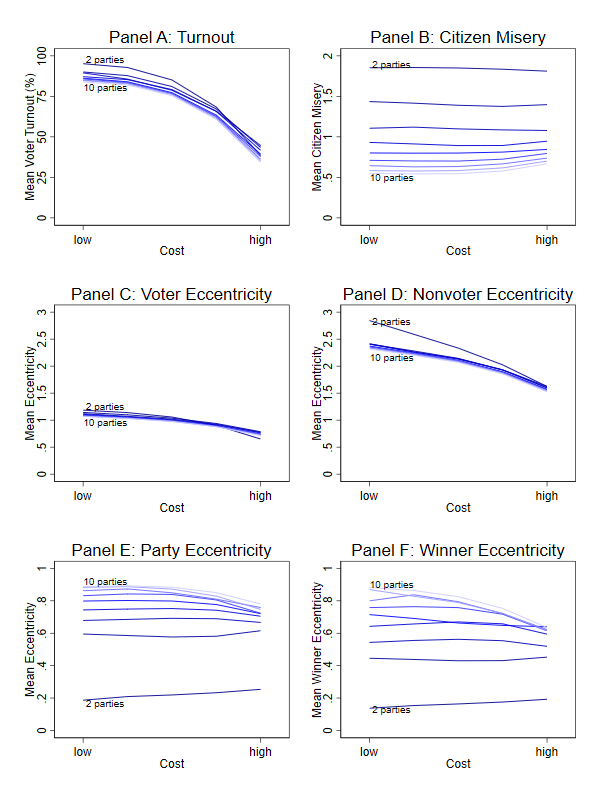
Panels C and D report voter and nonvoter eccentricity, which measures the location of the citizen relative to the median citizen. Overall citizen eccentricity — constant at \(1.25\sigma\) — can serve as an informative point of reference. By decomposing the eccentricity of all citizens into voters and abstainers, it reveals information about who abstains. Panel C shows that there are only small differences in the eccentricity of voters between party systems of different sizes, regardless of costs. In two and ten party systems at the lowest cost setting, where turnout is \(96.1\%\) and \(85.5\%\) respectively, voter eccentricity is very near the mean of the citizenry, and it declines as costs rise, suggesting that costs induce abstention at the extremes of the policy space. Panel D underscores this directly, revealing that as one increases costs, one adds abstainers ever closer to the median voter. Even so, they are never, on average, very close: at the highest cost, where average turnout is as low as \(34.2\%\) in the ten party case, the average abstainer is within \(2\sigma\) of the median citizen, but never closer than the average citizen at \(1.25\sigma\).
Turning now to properties of the parties, panel E reports party eccentricity, measured as the mean of the distance between the parties and the median citizen. One of the baseline (full turnout) results is that an increase in the number of parties increases party eccentricity; the results here show that this finding holds after introducing costly voting. However, they also reveal that the number of parties moderates the effect of voting costs on eccentricity. In small party systems, increasing costs leads to small increases in party eccentricity, while in large party systems, increasing costs lead to declining eccentricity. In two party systems, party eccentricity in the baseline full-turnout model is \(0.17\sigma\); when costs are at their highest (and turnout down to \(38.1\%\)), eccentricity is more than \(50\%\) higher, at \(0.26\sigma\).
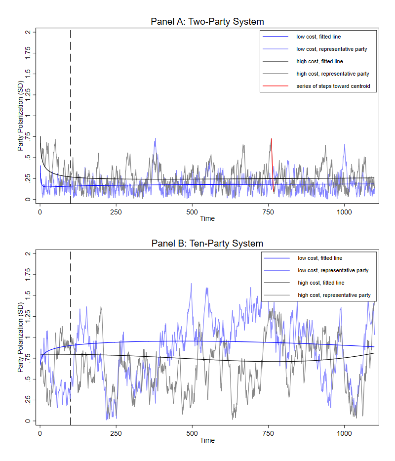
Figure 3 shows how individual vote-hunting parties adapt their location from moment to moment, even while system-level party eccentricity is in steady state over the long-run. Each time series plots the dynamics of one representative party over 1,100 time steps, together with fitted fractional polynomial lines, under four treatments created when the number of parties and the costs of voting take on their extreme values. The dashed vertical line in each panel demarcates the burn-in period prior to the 100th tick, during which the party is adapting from its random initialization location to the steady-state. Increasing segments of the lightly shaded observed values represent a series of steps away from the center, while declining segments represent steps towards the center. For example, the red segment in Panel A highlights a series of seven steps that this hunter took towards the center (in the two party, high-cost party system).
In Panel A with two parties, the party’s hunt for votes takes place relatively close to the center when voting costs are at their lowest, and relatively far when costs are at their highest. In Panel B with ten parties, the hunt takes place relatively far from the origin when voting costs are at their lowest, and relatively near when they are at their highest. Another notable distinction between the two panels is that the party’s hunt for voters around its own fitted line is tight in two party competition, and more varied in ten-party competition: hunters search locally for votes (taking one policy unit length step per tick), and in more crowded party systems, it takes longer for a party to find its way back to the steady state mean.
Finally, Panel F of Figure 2 reports the mean eccentricity of the winner relative to the median citizen. On average, the winner is always closer to the median citizen than the mean of all the parties; however, the winner is not always the least eccentric party in the party system. Under two party competition, the winner is closer to the median citizen than the average eccentricity of all the parties (and therefore closer than the only other party) more than \(93\%\) of the time. As costs increase, this percentage declines, ranging from a high of \(98\%\) under the lowest costs to a low of \(85\%\) under highest costs. As the number of parties increases, this percentage declines, and increasing costs has a less systematic effect. Under ten hunter competition, the winner is closer only \(55\%\) of the time, with a low of \(50\%\) when costs are low and a high of \(64\%\) when costs are high. In general, since hunters have a large stochastic element to their vote-seeking algorithm, and since election results depend upon the location and strength of parties, as well as the abstention decisions of citizens, winning positions can arise under diverse conditions. The diversity of these conditions increases as the number of parties and costs increase. The most we can say is that on average, the winning hunter is closer to the median citizen than the average of all the hunters, and that voting costs erode this tendency, especially in larger party systems.
All-aggregator competition
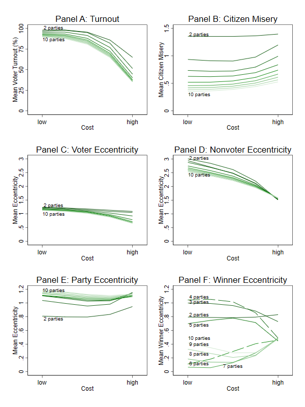
The all-aggregator results appear in Figure 4. In Panel A, turnout declines as voting costs and the number of parties increase. The lines fan out as they drop, showing that the negative effect of voting costs increases as the number of parties increases. Note further that all-aggregator party systems generate the highest average turnout across all treatments, compared with all-hunter and all-sticker party systems.
In Panel B, misery (i.e., the mean of the distance of each citizen to the nearest party) increases as costs rise, an effect which holds true in party systems of all sizes. The high cost observations deliver substantially higher misery to the citizenry, especially in larger party systems.
Panels C and D report the eccentricity of voters and abstainers relative to the median citizen at \((0, 0)\). The lowest cost observations are associated with mean turnout rates that range between 91.5% in ten-aggregator systems and 98.8% in two-party systems. With so few abstainers, the set of voters and the set of all citizens are very nearly the same, yielding eccentricity values near the mean citizen eccentricity value of \(1.25\sigma\). The abstainers in these cases arise as far as \(3\sigma\) from the origin in the two party case. Thus, as with the hunter models, abstention begins at the far extremes of the policy space. However, by the highest cost setting where turnout is as low as \(41.0\%\), there is no meaningful difference between the average eccentricity of the abstainers by party system size, indicating that they are arising throughout the policy space. In particular, the larger party systems generate earlier and more frequent centrist abstainers.
Panels E and F report party eccentricities relative to the median citizen. In Panel E, there are regularities at all but the highest cost observations. Specifically, mean party eccentricities increase as the number of parties increase. Increases in costs from the lowest values tend to lower mean eccentricity through moderate costs, before increasing eccentricity at the higher cost value. The high cost observations present anomalies also in other outcomes; I will return to them in the discussion.
Finally, Panel F in Figure 4 reports the mean eccentricity of the winner relative to the median citizen. The regularity reported above for all-hunter systems holds here, and is even stronger: on average, the winner is closer to the median citizen than the mean of all the parties in the system more than \(99\%\) of the time, except the four-aggregator system, when it is closer \(92\%\) of the time. Also, voting costs have a very small tendency to erode this propensity. However, Panel F reveals more interesting patterns.
The core to understanding these seemingly irregular patterns rests on two insights. The first insight considers only low cost voting. I begin by describing the pattern in Panel F. At low costs, winner eccentricity in two aggregator systems is approximately \(0.8\sigma\). From there, it increases for three and four party systems, before dropping to about \(0.7\sigma\) in five party systems. Beyond that, in larger party systems, winner eccentricity drops dramatically to about \(0.1\sigma\) for six and seven party systems, before rising again through the rest of the series until it hits about \(0.4\sigma\) in ten party systems.
These patterns have been examined formally in a field of computational geometry and are known as weighted CVTs, where the process that unfolds in our all-aggregator party competition is known as a convergence to a CVT stable state. In our models, and using the research design described in Section 4, we measure outcomes after the system arrives at this stable state.
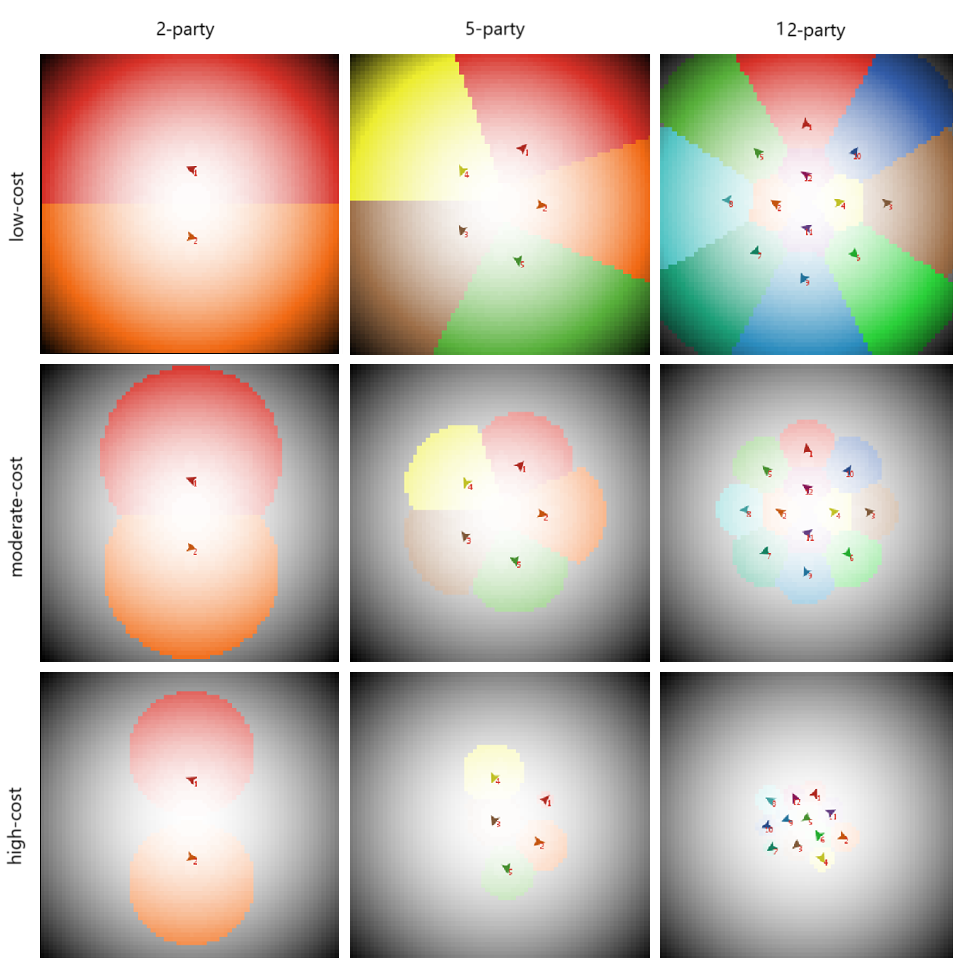
The physical distribution of the parties when there are two, three, and four parties is known as a “radially symmetric k-gon configuration,” where the parties arrange themselves as points at the circumference of a circle with a hollow center; the radius increases as the number of parties increases. At five parties, the system goes through the phase transition described in 3.6. The winner in a five party system takes an intermediate mean eccentricity because sometimes a fifth party moves to the center (with very low eccentricity), while on other repetitions the center remains hollow (with a relatively high eccentricity). A party in the center always wins. Finally, having passed through the phase transition, with six, seven, or more parties, one or more parties occupy the center and begin to form an inner ring. Computational geometers call these “multishell structures.” For a visual rendering of representative patterns, see the upper (low cost) row of Figure 5, where the two and five party cases are radially symmetric 2-gon and 5-gon configurations with a hollow center. The twelve party case is a multishell structure with eight parties around an outer ring, and four around an inner ring. These symmetric configurations describe the geometry of L&S’s baseline; their implications for, and relationship to, vote-share distributions observed in real elections are taken up in 6.7.
The second insight for understanding the patterns of Panel F concerns the impact of increases to the cost of voting. Higher costs undermine the ability of the set of all-aggregator algorithms to minimize misery by forming a CVT. In the second row of images in Figure 5, where costs are moderate, the partitions seem to retain the geometric regularity of the low cost case, despite the presence of abstainers at the periphery. However, by the highest cost setting, with abstainers appearing at central locations between parties, the regularity of the pattern breaks down and the gap sizes between parties grow uneven.
Discussion and Conclusion
This study advances theoretical models of party competition by introducing voting costs and examining the system-level implications. By relaxing the assumption of costless voting in the standard spatial model, it reveals interdependency between electoral participation, party behavior, and the broader political system.
The models offer several significant results, all from a baseline which replicates the no-cost results in chapter five of L&S. First, higher voting costs consistently suppress voter turnout across all scenarios, though the effect size varies by the number of parties and the type of party system. This result a) establishes voting costs as a viable mechanism for operating on turnout; b) establishes a fruitful integration of two classical models — the spatial model and the calculus of voting model — within a computational setting; and c) sets the foundation to study the nature of and follow-on consequences of abstention.
Second, the interaction between voting costs and the number of parties yields complex patterns of party eccentricity. The big story in the all-hunter results builds from what we know from the median voter theorem and L&S: that two-hunter competition and no costs yields party convergence towards the median citizen, and that increasing the number of parties increases party divergence. Set against this background, there are two surprises: in two-party competition, hunters diverge from the median as costs increase; and in large party systems, parties converge as costs increase.
The mechanisms that give rise to these adaptations are as follows. In small hunter systems, abstention at the periphery pulls parties outward, since peripheral steps now yield vote-share gains by recapturing newly abstaining citizens. This outward movement comes at the cost of more moderate citizens, who begin to abstain along the boundaries between parties where they are approximately indifferent between adjacent parties’ positions. A party’s tendency on average toward greater eccentricity stops when the votes gained at the periphery balance the votes lost closer to the center. This balance between centripetal and centrifugal forces is another instance of the stigmergic coordination introduced in 4.10: parties coordinate their long-run spatial positions through the shared environment of the citizenry’s voting and abstention decisions, without any party being aware of, or directly responding to, the others. In large hunter systems, the same stigmergic logic produces different dynamics. Abstention is still densest at the periphery, but with high voting costs it also extends inward along the boundaries between parties, where moderate citizens are approximately indifferent between adjacent parties. On average, hunters in large party systems balance their gains and losses by settling closer to the median citizen. The centrifugal dynamic identified here for small hunter systems is consistent with recent formal models of voting costs and polarization (Oprea et al. 2024; Sasso et al. 2022).
Similar patterns arise in the all-aggregator scenario; however, the aggregator strategy is a newer and less-studied heuristic with weaker priors about what to expect. Overall, and together with other findings, there is evidence that costs shape the spatial positioning of parties, and that they operate through adaptive behaviors that are responding to the patterns of abstention in the citizenry.
Third, voting costs sometimes undermine citizen representation, especially in multi-party systems. The big story here arises in the all-aggregator scenario, where we know from L&S that the aggregator heuristic in the full-turnout setting optimizes representation when all parties use it. Indeed, they note that the aggregator heuristic generalizes to Lloyd’s algorithm (Lloyd 1982), with origins in mathematics and electrical engineering, suggesting that there may be further insights to exploit from other disciplines. Set against this background, I find that the forces that generate this regularity completely break down under the highest costs, when (as seen in Figure 5) abstention has spread from alienated citizens at the periphery of the policy space to indifferent citizens between the parties — sometimes referred to as abstention due to indifference. Aggregators, who are content to represent their current voters, do not seek abstainers who may exist in high density regions of the policy space; instead, when costs are high they often become small islands of representation surrounded by the open seas of abstention.
This breakdown of the all-aggregator CVT under costly voting has a further implication. The symmetric vote-share configurations visible in the no-cost baseline rows of Figure 5 — five parties at roughly equal shares, twelve parties in a clean multishell structure — pertain to the L&S baseline, designed to isolate party-system behavior when parties are homogeneous in their strategy. Real party systems rarely look this way. Election contests in majoritarian constituencies (i.e., in single-member district plurality systems) routinely produce 60–40 or 75–25 margins, and multi-party systems typically have a few major parties accompanied by many smaller parties. Features in real political systems that explain these observed asymmetries — such as mixed party strategies and non-Normal distributions of citizen policy preferences — are treated in empirical analyses of L&S Chapter 11 and Laver (2005). The contribution of the present paper is complementary. Within the L&S baseline, where these features are switched off by construction, the introduction of voting costs alone is sufficient to disrupt the symmetric prediction. Visually, this appears as the progressive collapse of the CVT in the lower rows of Figure 5; in aggregate, it also appears as the gap between the effective and absolute number of parties at high costs in Figure 8. Costly voting therefore stands alongside other features as a mechanism the baseline framework had not previously identified for explaining departures from equal vote shares in multi-party systems.
These results have several theoretical and practical implications. Theoretically, this study bridges gaps between spatial models of party competition and behavioral theories of turnout by integrating costs into the modeling of party competition. This integration allows for a richer exploration of real-world phenomena such as voter disenfranchisement, strategic voter abstention, and the trade-offs inherent in multi-party systems. Normatively, the results bring to light the consequences of institutional or contextual factors that increase voting costs, such as voter identification laws, which were recently adopted in the United Kingdom. Depending upon the type of parties in a party system, such barriers — apart from the stated goal of increasing election security — may unintentionally reduce participation and representation while exacerbating polarization.
This work opens avenues for further inquiry. First, from within the framework of L&S, other specifications beyond the chapter 5 baseline models call for an examination of the influence of voting costs. It makes sense to start with their baseline models, but major contributions of the book arise in subsequent chapters using models which place different party strategies in competition with each other, and models that allow for endogenous party birth and death. Will voting costs influence the relative fitness of different party strategies in the tournament-style competition they build?
Second, where here I assume that all citizens face homogeneous costs, future work can incorporate heterogeneous costs that reflect, for example, socio-economic disparities, or that arise endogenously from electoral competition.
Third, by introducing voting costs and endowing citizens with more capabilities, models can be developed that investigate more nuanced party strategies, including ones which operate on the cost of voting (i.e., vote-buying) and other non-policy appeals such as populist and clientelist party-voter linkage strategies (Lehrer & Schumacher 2018; Reinermann 2014). In recent decades, a great deal of interest in political science has arisen around the study of these non-policy party strategies. Aldrich uses the calculus of voting model to theorize about party strategy with his “strategic party hypothesis” (1995). He notes that in contrast to citizens (who encounter very small marginal costs and benefits from voting), parties care deeply about electoral outcomes: “It is thus strategic political leaders who strategize more ‘deeply’, seeking to manipulate the [terms of the calculus of voting model] to enhance turnout…” (1997 p. 388). Building upon this, several scholars have developed a basis for more diverse party-voter linkage strategies using the calculus of voting model, as for example by deriving symbolic, clientelist, and vote-buying party strategies (Mustillo 2016). These ideas can be transformed into party algorithms and citizen utility functions, and thereby further loosen the assumption that all politics is spatially-oriented.
Finally, there is a great need for empirically grounded research to validate the associations between the main input and outputs in these models, as well as work to explore the mechanisms linking them (Muis 2010; Troitzsch 2021). Calibrated, mixed-rule extensions of the costly-voting model to real party systems would directly engage the question of how voting costs interact with the strategic and citizen distribution heterogeneities that produce the unequal vote shares observed in real elections. Work along these lines, applied to the British case using British Election Study panel data and exploiting the 2023 introduction of mandatory voter identification, is under development.
The computational exploration of costly voting enriches our understanding of the dynamics of party competition and voter behavior. By demonstrating how participation costs cascade through the political system, this study contributes to ongoing debates about electoral integrity, party strategy, and democratic representation. Addressing the barriers to participation remains essential for fostering inclusive and responsive political systems.
Acknowledgements
I am grateful for support from Abhi Deshmukh, research assistance from David Dalenberg, David Dalenberg, Yuvaraj Pazhamalai, and for comments from participants in meetings at the Midwest Political Science Association, Notre Dame’s Kellogg Institute Working Paper Series, and the Université de Montréal’s Centre de Recherches Mathématiques, as well as from anonymous referees.Notes
- Other computational approaches that treat abstention include Fieldhouse et al. (2016) and Kottonau & Pahl-Wostl (2004).↩︎
- These include: “issue owners” who build credibility on subsets of issues (Reinermann 2014); “predators” who attack popular parties (Laver 2005); “governators” who seek to join governing coalitions (Lehrer & Schumacher 2018); and 25 other algorithms that were submitted for a tournament of party competition (Fowler & Laver 2008).↩︎
- In other computational models, the electorate considers other features. For example, Reinermann (2014) introduces voter consideration of the past, and of personal qualities of party leaders. Fowler & Smirnov (2005) develops a model of “social turnout” in which citizens are responsive to the turnout decisions of other citizens. L&S also treat non-policy motivations as a model extension.↩︎
- In order to replicate the baseline full turnout models published in L&S and reported here in Appendix A, I set cost to an arbitrarily low value of \(C = -10000\) to generate nearly full turnout under all circumstances.↩︎
Appendix A: Replication of L&S Full Turnout (No-Cost) Results
The results in Figure 6 arise when costs are set to -10,000, which is an arbitrarily low value to approximate full turnout. Very small deviations from full turnout arise occasionally. Mean turnout for all-hunter, all-aggregator, and all-sticker runs are 99.92%, 99.92%, and 99.90%, respectively.
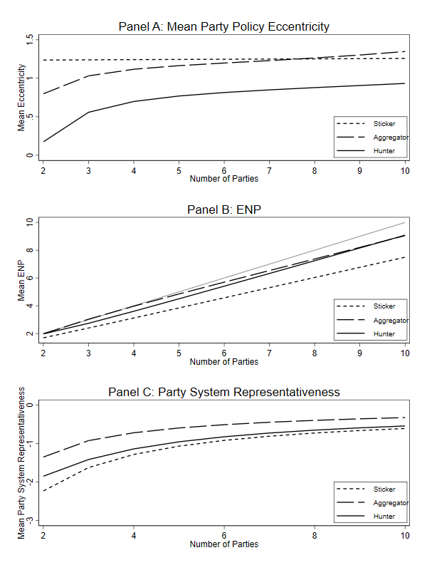
Panel A shows mean party eccentricity and replicates Figure 5.2 in L&S. Panel B shows mean ENP and replicates Figure 5.5. Panel C shows mean party system representativeness and replicates Figure 5.6.
The results here replicate, with two trivial differences that arise from different operationalizations. First, party system representativeness in L&S is the additive inverse of citizen misery, which I use here. These are conceptually related in the sense that representativeness defines the concept in terms of the parties, whereas misery defines the concept in terms of the citizens. When party system representativeness is at a maximum of 0 (each citizen has its own party), citizen misery is at a minimum of 0. As the mean distance between each citizen and the nearest party increases, representativeness decreases, and misery increases.
Second, in my model, initial party locations are distributed normally in two dimensions around the median citizen, and with a standard deviation of 10 policy units, whereas L&S’s replication file for their chapter 5 models—available at the NetLogo Modeling Commons—initializes the parties using a routine that does not generate a bivariate normal distribution (even though the annotation in the codes indicates that it does). The mean distance from the center under the Normal distribution is approximately 12.5 policy units. Their implementation is as follows: first, parties are born at the center; then, they choose a random heading between 0 and 360 degrees; finally, they take a step of a size drawn randomly between values of 0 and 30. This results in a uniform distribution of step sizes, with a mean of 15. Thus, in their results, the mean party eccentricity in the all-sticker model is \(1.5\sigma\).
Appendix B: Results of All-Sticker Models
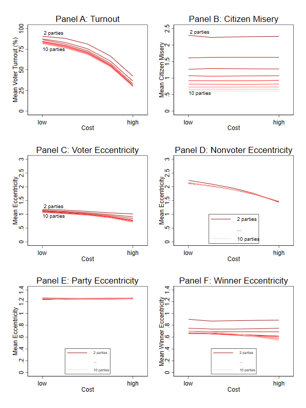
Results for all-sticker models are less interesting, but I report them for completeness since they are reported in chapter 5 of L&S. In Figure 7, Panel A, turnout declines as voting costs and the number of parties increase. Panel B shows that costs have no effect on citizen misery (because parties do not adapt). Misery declines as a function of the number of parties because with each new party, at least a small cluster of citizens receives a new preferred party (i.e., a closer party). In Panels C and D, abstainers first begin to arise at the extremes of the policy space, and become increasingly moderate (on average) as costs increase. Panel E, which shows mean party eccentricity constant at \(1.25\sigma\), simply reflects the randomization process of the party initialization process, which distributes parties at a location drawn randomly from a bivariate Normal distribution centered at \((0,0)\) and with a standard deviation of \(10\) units. Panel F shows that winners are closer than the party system mean eccentricity, and that voting costs have little or no effect.
Appendix C: Results for Effective Number of Parties
Results for the effective number of parties (ENP) are of less interest, but I report them for completeness since they are reported in chapter 5 of L&S.
This outcome is defined by Laakso & Taagepera (1979) as a concept that taps the fragmentation of the party system and answers the question: how equally is the vote distributed among the parties in the system? The measure, \(ENP\), amounts to a count of the parties, weighted by their vote share
| \[ENP = \frac{1}{\sum_{p=1}^{j} e_j^2}\] | \[(14)\] |
It has a theoretical minimum of \(1\) (when all votes go to a single party), and a maximum equal to the number of parties (when the vote share is divided equally between them).
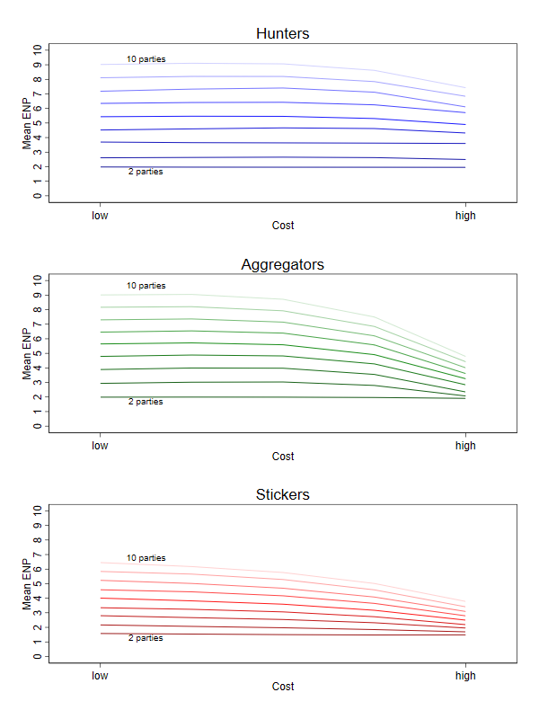
L&S find only very small departures from equality in party vote shares under full turnout for hunters and aggregators, a result repeated here under the lowest costs. Figure 8 shows that as costs increase, inequality in the vote shares increases (i.e., ENP declines), with larger effects as the number of parties increases.
References
ADAMS, J. F., Merrill III, S., & Grofman, B. (2005). A unified theory of party competition: A cross-national analysis integrating spatial and behavioral factors. Cambridge: Cambridge University Press. [doi:10.1017/cbo9780511614453]
ALDRICH, J. H. (1995). Why Parties?: The Origin and Transformation of Political Parties in America. Chicago, IL: University of Chicago Press.
ALDRICH, J. H. (1997). When is it rational to vote? In D. C. Mueller (Ed.), Perspectives on Public Choice: A Handbook. Cambridge: Cambridge University Press.
BENDOR, J., Diermeier, D., & Ting, M. (2003). A behavioral model of turnout. American Political Science Review, 97(2), 261–280. [doi:10.1017/s0003055403000662]
BAKKER, R., Jolly, S., & Polk, J. (2012). Complexity in the European party space: Exploring dimensionality with experts. European Union Politics, 13(2), 219–245. [doi:10.1177/1465116512436995]
BENOIT, K., & Laver, M. (2006). Party Policy in Modern Democracies. London: Routledge. [doi:10.4324/9780203028179]
BRODY, R. A., & Page, B. I. (1973). Indifference, alienation and rational decisions: The effects of candidate evaluations on turnout and the vote. Public Choice, 15, 1–17. [doi:10.1007/bf01718840]
CHEN, T. H. (2011). Uncovering the micro-foundations of turnout and electoral systems. Electoral Studies, 30(2), 295–308. [doi:10.1016/j.electstud.2011.01.001]
DE Marchi, S. (1999). Adaptive moDEls and electoral instability. Journal of Theoretical Politics, 11(3), 393–419. [doi:10.1177/0951692899011003007]
DOWNS, A. (1957). An Economic Theory of Democracy. New York, NY: Harper; Row.
DE MARCHI, S. (2003). A computational model of voter sophistication, ideology, and candidate position-taking. In K. W. Kollman, J. H. Miller, & S. E. Page (Eds.), Computational Models in Political Economy. Cambridge, MA: The MIT Press. [doi:10.7551/mitpress/2021.003.0007]
DU, Q., Faber, V., & Gunzburger, M. (1999). Centroidal Voronoi tessellations: Applications and algorithms. SIAM Review, 41(4), 637–676. [doi:10.1137/s0036144599352836]
FIELDHOUSE, E., Green, J., Evans, G., Mellon, J., Prosser, C., Geus, R. de, & Bailey, J. (2024). 2019 British Election Study Post-Election Random Probability Survey.
FIELDHOUSE, E., Lessard-Phillips, L., & Edmonds, B. (2016). Cascade or echo chamber? A complex agent-based simulation of voter turnout. Party Politics, 22(2), 241–256. [doi:10.1177/1354068815605671]
FOWLER, J. H., & Laver, M. (2008). A tournament of party decision rules. Journal of Conflict Resolution, 52(1), 68–92. [doi:10.1177/0022002707308598]
FOWLER, J. H., & Smirnov, O. (2005). Dynamic parties and social turnout: An agent-based model. American Journal of Sociology, 110(4), 1070–1094. [doi:10.1086/426554]
GEYER, L., & Mellacher, P. (2025). Simulating party competition in dynamic voter distributions. GSC Discussion Paper Series, Paper No. 32
GRIMM, V., Berger, U., DeAngelis, D. L., Polhill, J. G., Giske, J., & Railsback, S. F. (2010). The ODD protocol: A review and first update. Ecological Modelling, 221(23), 2760–2768. [doi:10.1016/j.ecolmodel.2010.08.019]
HARTIGAN, J. A., & Wong, M. A. (1979). Algorithm AS 136: A K-Means Clustering Algorithm. Applied Statistics, 28(1), 100. [doi:10.2307/2346830]
HESS, S. W., Weaver, J. B., Siegfeldt, H. J., Whelan, J. N., & Zitlau, P. A. (1965). Nonpartisan political redistricting by computer. Operations Research, 13(6), 998–1006. [doi:10.1287/opre.13.6.998]
HOTELLING, H. (1929). Stability in competition. The Economic Journal, 39, 41–57.
JACKSON, J. E. (2003). A computational theory of electoral competition. In K. W. Kollman, J. H. Miller, & S. E. Page (Eds.), Computational Models in Political Economy. Cambridge, MA: The MIT Press. [doi:10.7551/mitpress/2021.003.0006]
KOLLMAN, K., Miller, J. H., & Page, S. E. (1992). Adaptive parties in spatial elections. American Political Science Review, 86(4), 929–937. [doi:10.2307/1964345]
KOLLMAN, K., Miller, J. H., & Page, S. E. (1998). Political parties and electoral landscapes. British Journal of Political Science, 28(1), 139–158. [doi:10.1017/s0007123498000131]
KOTTONAU, J., & Pahl-Wostl, C. (2004). Simulating political attitudes and voting behavior. Journal of Artificial Societies and Social Simulation, 7(4), 6.
LAAKSO, M., & Taagepera, R. (1979). The effective number of parties: A measure with application to Western Europe. Comparative Political Studies, 12(1), 3–27. [doi:10.1177/001041407901200101]
LAVER, M. (2005). Policy and the dynamics of political competition. American Political Science Review, 99(2), 263–281. [doi:10.1017/s0003055405051646]
LAVER, M., & Sergenti, E. (2012). Party Competition: An Agent-Based Model. Princeton, NJ: Princeton University Press. [doi:10.23943/princeton/9780691139036.001.0001]
LEHRER, R., & Schumacher, G. (2018). Governator vs. Hunter and Aggregator: A simulation of party competition with vote-seeking and office-seeking rules. PLoS One, 13(2), e0191649. [doi:10.1371/journal.pone.0191649]
LLOYD, S. (1982). Least squares quantization in PCM. IEEE Transactions on Information Theory, 28(2), 129–137. [doi:10.1109/tit.1982.1056489]
LORENZ, J., Neumann, M., & Schröder, T. (2021). Individual attitude change and societal dynamics: Computational experiments with psychological theories. Psychological Review, 128(4), 623–642. [doi:10.1037/rev0000291]
MACQUEEN, J. B. (1967). Some methods of classification and analysis of multivariate observations, Proceedings of the 5th Berkeley Symposium on Mathematical Statistics and Probability.
MUIS, J. (2010). Simulating political stability and change in the Netherlands (1998-2002): An agent-based model of party competition with media effects empirically tested. Journal of Artificial Societies and Social Simulation, 13(2), 4. [doi:10.18564/jasss.1482]
MUSTILLO, T. (2016). Party-voter linkages derived from the calculus of voting model: Electoral mobilization in Ecuador. Rationality & Society, 28(1), 24–51. [doi:10.1177/1043463115621516]
NOWAK, M., & Sigmund, K. (1993). A strategy of win-stay, lose-shift that outperforms tit-for-tat in the Prisoner’s Dilemma game. Nature, 364(6432), 56–58. [doi:10.1038/364056a0]
OPREA, A., Martin, L., & Brennan, G. H. (2024). Moving toward the median: Compulsory voting and political polarization. American Political Science Review, 118(4), 1951–1965. [doi:10.1017/s0003055423001399]
REINERMANN, H. (2014). Party competition and voter decision-making. Advances in Computational Social Science and Social Simulation
RIKER, W. H., & Ordeshook, P. C. (1968). A theory of the calculus of voting. American Political Science Review, 62(1), 25–42. [doi:10.2307/1953324]
ROYSTON, P., & Altman, D. G. (1994). Regression using fractional polynomials of continuous covariates: Parsimonious parametric modelling. Journal of the Royal Statistical Society. Series C (Applied Statistics), 43(3), 429–467. [doi:10.2307/2986270]
SASSO, G., Judd, G., & Steel, R. (2022). Electoral competition with targeted voting costs. [doi:10.31235/osf.io/gsb3r]
SCHEDLER, A. (2023). Rethinking political polarization. Political Science Quarterly, 138(3), 335–359. [doi:10.1093/psquar/qqad038]
SCHUMACHER, G., & Vis, B. (2012). Why do social democrats retrench the welfare state? A simulation. Journal of Artificial Societies and Social Simulation, 15(3), 4. [doi:10.18564/jasss.1959]
STATACORP. (2019). Stata Statistical Software: Release 16. College Station, TX.
TROITZSCH, K. G. (2021). Validating simulation models: The case of opinion dynamics. In T. Rudas & G. Péli (Eds.), Pathways Between Social Science and Computational Social Science (pp. 123–155). Springer International Publishing. [doi:10.1007/978-3-030-54936-7_6]
WILENSKY, U. (1999). NetLogo. Center for Connected Learning and Computer-Based Modeling, Northwestern University, Evanston, IL
WRIGHT, M., & Sengupta, P. (2015). Modeling oligarchs’ campaign donations and ideological preferences with simulated agent-based spatial elections. Journal of Artificial Societies and Social Simulation, 18(2), 3. [doi:10.18564/jasss.2736]