Calibrating a Global Trade Agent-Based Model with an HPC–ABC–SMC Framework

, ,
and
aUniversity of Leeds, Great Britain; bUniversity of Leeds, United Kingdom; cThe James Hutton Institute, United Kingdom
Journal of Artificial
Societies and Social Simulation 29 (3) 5
<https://www.jasss.org/29/3/5.html>
DOI: 10.18564/jasss.6072
Received: 17-Sep-2025 Accepted: 22-Jun-2026 Published: 30-Jun-2026
Abstract
This study presents a High-Performance Computing and Approximate Bayesian Computation-Sequential Monte Carlo (HPC-ABC-SMC) framework for calibrating complex agent-based models. Applied to a global food trade model, the framework calibrates trade partner and trade volume objectives separately, using precomputed result mapping and task-level parallelisation to achieve up to a 42.1-fold computational efficiency improvement over traditional methods. Unlike conventional optimisation approaches, our method provides posterior distributions rather than single-point estimates, enabling richer interpretation of parameter uncertainty. The results reveal systematic differences between partner-based and volume-based calibrations: partner calibration yields smaller parameter magnitudes due to higher sensitivity, while volume calibration requires larger weights under looser constraints. Comparative analysis shows consistency with genetic algorithms but demonstrates superior interpretability, while sensitivity analysis highlights the dominant role of GDP per capita weight in shaping international trade patterns. Overall, the framework offers a scalable and uncertainty-aware solution for calibrating empirical agent-based models with high-dimensional parameter spaces and alternative evaluation criteria.Introduction
Agent-Based Models (ABMs) have become a powerful tool for simulating complex adaptive systems across a wide range of disciplines. In the social sciences, ABMs have been widely used to study collective behaviour, social interactions, and institutional dynamics (Bianchi & Squazzoni 2015; Verhagen et al. 2021). In ecology and social-ecological systems research, they enable the simulation of multi-scale interactions between human actors and natural environments (Ekström et al. 2024; Lippe et al. 2019). In economics and finance, they capture market dynamics, systemic risk, and emergent macroeconomic phenomena (Axtell & Farmer 2025). Their shared strength lies in representing heterogeneous agents and capturing emergent system-level dynamics, making them particularly suitable for studying complex phenomena such as global trade systems, resource allocation, and policy interventions. As ABMs increase in complexity in order to better reflect empirical realities (Sun et al. 2016), parameter calibration and uncertainty quantification become increasingly challenging. While calibration is not always required for conceptual exploration, it is essential for models aiming to achieve empirical validity or support data-informed policy analysis (Gilbert et al. 2018).
A central difficulty in Bayesian calibration of ABMs lies in computational scalability. Most existing Approximate Bayesian Computation (ABC) workflows tightly couple the statistical sampler with the ABM platform through interface-based execution. For NetLogo models, tools such as BehaviorSpace, PyNetLogo, RNetLogo, nlrx, and nl4py enable batch simulation from Python or R environments(Gunaratne & Garibay 2021; Jaxa-Rozen & Kwakkel 2018; Salecker et al. 2019; Thiele et al. 2012). However, these approaches typically require repeated interface-based invocations of the model, which incur serialization overhead, limit effective parallelization, and may constrain the use of certain NetLogo extensions in high-performance computing (HPC) environments.
Beyond interface overhead, calibration of computationally intensive ABMs demands thousands of simulation runs across high-dimensional parameter spaces (Platt 2020). In tightly coupled workflows, each ABC-SMC iteration repeatedly calls the simulator, amplifying communication costs and reducing scalability. In our implementation, the NetLogo Python Extension was found to be incompatible with PyNetLogo due to conflicts between the embedded JVM and the external Python process[1], further motivating the adoption of direct headless execution on the HPC cluster. As a result, Bayesian calibration of computationally intensive ABMs remains demanding, limiting broader adoption in applied socio-economic modelling.
To address this structural bottleneck, this study introduces a precomputed result mapping strategy within an HPC-enabled ABC-SMC framework—the central methodological contribution of this work. Instead of invoking the ABM through interfaces at each inference step, the proposed architecture decouples simulation execution from statistical inference. The calibration workflow separates into two stages per ABC-SMC generation: (1) batch execution of all required NetLogo simulations as independent HPC tasks, with outputs aggregated into a parameter–output lookup table; and (2) local ABC-SMC inference that queries this lookup table without invoking NetLogo. This decoupling eliminates repeated interface overhead and enables true task-level parallelization across simulation batches.
Applied to a global trade ABM with three calibration parameters across 8–10 ABC-SMC generations, the framework achieves up to a 42-fold reduction in wall-clock time compared to GUI-based single-core execution, while providing full posterior distributions for comprehensive parameter uncertainty quantification. The study demonstrates how this architecture can scale Bayesian calibration for computationally intensive ABMs and provides a generalizable solution for likelihood-free inference in models supporting batch execution.
Background
Despite the strong analytical capabilities of agent-based modeling, it faces significant challenges in parameter estimation and uncertainty quantification (Lee et al. 2015). As model complexity increases, the parameter space grows exponentially, making exhaustive exploration computationally prohibitive (Carrella 2021). This challenge is especially pronounced in high-dimensional and stochastic models, where identifying parameter combinations that reproduce observed patterns is a complex process (Grimm et al. 2005; Windrum et al. 2007). Carrella (2021) highlights that estimation algorithms perform inconsistently across models and even within the same model, with optimal methods varying by parameter. Selecting an unsuitable algorithm can significantly increase computational costs, rendering it impossible for quantitative calibration.
Existing parameter calibration methods may perform well on simplified, prototype models but are often limited in more complex real-world applications, as simple models are generally easier to estimate successfully (Carrella 2021). A related challenge concerns the choice of summary statistics: when modelers compress full ABM output into a lower-dimensional set of summary statistics—often driven by computational constraints—the resulting statistics may be insufficiently informative. In such cases, a wide range of parameter combinations can produce identical summary values, rendering some parameters effectively non-identifiable. Increasing the informativeness of the summary statistics can substantially improve estimation performance without changing the underlying model output (Beaumont 2019). These concerns reinforce doubts about the applicability of many calibration algorithms to large-scale, high-dimensional ABMs (Carrella 2021; Platt 2020).
High-performance computing (HPC) is crucial for improving the execution efficiency of NetLogo models, enabling large-scale model experiments to be conducted on HPC clusters or desktop computers. Even computationally intensive models can be executed thousands of times. Additionally, NetLogo supports tools such as BehaviorSearch and RNetLogo, which assist in designing and managing large-scale experiments by automating parameter exploration and batch simulation workflows (Railsback et al. 2017).
In recent years, parameter calibration based on Bayesian inference, particularly Approximate Bayesian Computation (ABC), has garnered widespread attention due to its ability to quantify the uncertainty in parameter estimation (Grazzini et al. 2017). However, applying ABC in agent-based modeling (ABM) research typically requires a large number of simulation runs, making computational efficiency a critical challenge. To address this issue, researchers have explored the use of surrogate models to accelerate the simulation process and reduce computational costs. Machine learning approaches, such as Random Forest and Generalized Additive Models, have been employed to improve efficiency. While these methods can enhance computational performance in certain scenarios, they still face limitations when dealing with high-dimensional ABM parameter calibration. Moreover, their simulation accuracy often falls short of that achieved by the original model (Lamperti et al. 2018; Vaart et al. 2015). Although direct simulation using the original model is computationally more expensive, it provides more accurate and reliable results, which is particularly crucial for studying the nonlinear dynamics of real-world applications. A pressing research challenge is how to effectively integrate large-scale, computational simulations with advanced statistical algorithms, such as Bayesian inference, for robust parameter estimation.
NetLogo provides several useful features for experiment management, including independent parameter execution, conditional measurement recording, and XML-based import/export for headless runs (Wilensky 2023). Among these, the built-in tool BehaviorSpace supports batch experiments and parameter sweeps. However, it lacks flexibility for adaptive calibration and is not well suited for high-dimensional parameter tuning or large numbers of parallel simulation tasks in high-performance computing (HPC) environments. These limitations motivate the need for more specialised solutions that enable dynamic parallel task management and iterative parameter adaptation.
In this study, we leverage NetLogo’s XML functionality to batch-write parameters into predefined experiment configuration files, enabling automated parameter generation and HPC-based parallel simulation execution. Simulation results are then integrated into the ABC framework, forming an iterative calibration process in which the local environment reads simulation outputs, generates the next generation of parameter sets, and repeats the procedure until convergence.
ABC-Sequential Monte Carlo (ABC-SMC), a variant of the ABC method, enhances parameter search efficiency and uncertainty quantification through a population-based sequential sampling scheme (Toni et al. 2009). Compared to standard ABC, ABC rejection sampling becomes highly inefficient when there is a large discrepancy between the target posterior and prior. Another commonly used variant is ABC with Markov Chain Monte Carlo (MCMC) sampling, where Markov chains are used to explore the parameter space based on posterior similarity. MCMC is a general technique for drawing samples from complex posterior distributions, and in the context of ABC, it enables more focused exploration without evaluating the exact likelihood. Although this approach is generally more efficient than rejection sampling, it may suffer from poor mixing and slow convergence in high-dimensional parameter spaces (Wang et al. 2024). (Thiele et al. 2012) also noted that ABC is the ideal technique, but its high computational cost may make it impractical for large, computationally expensive models.
More recently, neural simulation-based inference (SBI) methods have
emerged as a promising alternative for likelihood-free Bayesian
calibration of ABMs. Approaches such as neural posterior estimation
(NPE) and neural density-ratio estimation (NRE) train neural networks to
approximate the posterior distribution directly from simulated data, and
have been successfully applied to economic and financial ABMs (Dyer et al. 2024; Platt
2022). A publicly available implementation,
sbi4abm, further facilitates adoption and is naturally
amenable to HPC parallelization. However, these approaches typically
require large numbers of simulations for network training, and their
performance can be sensitive to the choice of network architecture and
summary statistics. In contrast, ABC-SMC operates directly on simulation
outputs without requiring a training phase, making it more
straightforward to implement and interpret in applied calibration
settings with constrained simulation budgets.
Existing research demonstrates the significant time efficiency of HPC clusters in parallelizing and executing large-scale simulation experiments (Railsback et al. 2017). However, current Python statistical libraries, such as PyABC (Klinger et al. 2018), face challenges in integrating with NetLogo models, particularly due to limitations in direct interaction and the utilization of HPC multi-threading capabilities. To address this gap, this study presents a framework that integrates HPC computing resources and ABC-SMC statistical inference for objective-specific calibration. By leveraging precomputed simulation outputs within the PyABC workflow, the framework circumvents performance bottlenecks associated with repeated API-based model interactions, thereby significantly improving computational efficiency and enabling the effective execution of computationally intensive simulation experiments.
Methodology
Overview of the agent-based model
To demonstrate the effectiveness of our proposed calibration framework, we first develop and validate the approach, and then apply it to a complex and data-rich ABM of global trade. This application serves as a proof-of-concept for calibrating high-dimensional, multi-objective ABMs using scalable Bayesian techniques. The selected model is particularly suitable as a test case because it features multiple interacting agents, a large number of tunable parameters, and diverse output indicators—characteristics that typify the calibration challenges in real-world ABM applications.
Specifically, we build on the Relation-Driven Agent-Based Global Trade Model introduced in (Ge et al. 2021), extending and applying it to the issue of food and nutrition security. The model adopts a relationship-driven perspective and employs agent-based methods to depict the dynamic interactions among countries (or regions) in the international trade network, while simulating grain production, consumption demand, and trade strategies. A key feature of the model is its ability to capture complex relationships in trade behavior through multidimensional, multi-scale data and parameters.A concise description of the model structure and key behavioural rules, following the ODD protocol, is provided in Appendix A.
In this research, we update the original framework by refreshing the historical data coverage from 2000–2013 to 2010–2022, and recalibrate the following parameters in Table 1. While the agent-based model is designed to run from 2010 to 2050 in order to support long-term scenario exploration, the calibration in this study is deliberately restricted to the years 2011–2017. This decision reflects both the availability and reliability of empirical trade and food balance data during this period, as well as the need to ensure consistent evaluation metrics. In practice, the longer-term horizon (2018–2050) is used for forward-looking simulations and policy scenarios, whereas the calibration stage focuses on aligning the model with observed historical patterns.
| Parameter Name | Description | Parameter Range |
|---|---|---|
| Per Capita GDP Weight | Reflects the influence of economic strength on trade priorities | 0.05 – 20 |
| Geographic Distance Weight | Fixed at 1, serving as the baseline for other parameters | 1 (fixed) |
| Historical Trade Relationship Weight | Represents the reinforcing effect of long-term cooperation on trade tendencies | 0.05 – 20 |
| Emerging Trade Relationship Weight | Characterizes how random events lead to path dependency in subsequent trade flows | 0.05 – 20 |
In the model, each country is represented as an agent that makes trade decisions based on economic capacity, geographic constraints, and historical trade relationships. At each simulation step, countries evaluate potential trading partners using a weighted ranking mechanism that incorporates GDP per capita, geographic distance, and both historical and emerging trade relationships. Trade flows are generated through an iterative matching process between importing and exporting countries, allowing the global trade network to evolve dynamically over time.
Model Evaluation Metrics
Model performance is evaluated using two empirical indicators:the trade volume match rate and the trade partner match rate.These metrics assess the extent to which the simulated trade system reproduces observed international trade patterns in terms of both trade quantities and network structure.
Trade volume match rate
The trade volume match rate evaluates how well the simulated trade volumes (imports, exports, and food consumption) align with actual data from FAO Food Balance Sheets (FBS). A match is considered if at least one of the three trade categories (import, export, or food consumption) falls within ±20% of its actual value.
The trade volume match rate is then computed as the percentage of country-year records that meet this condition over the evaluation period (2011–2017): \[\begin{equation} \text{Matching Rate of Trade Volume} = \frac{1}{C} \sum_{c=1}^{C} \frac{1}{T} \sum_{t=2011}^{2017} \mathbb{1} \left( \left| \frac{V_{c,t}^{\text{sim}} - V_{c,t}^{\text{real}}}{V_{c,t}^{\text{real}}} \right| \leq 0.2 \right) \end{equation}\] where \(C\) is the total number of countries, \(T = 7\) represents the years evaluated, and \(\mathbb{1}(\cdot)\) is an indicator function that returns 1 if at least one trade category meets the condition, otherwise 0.
Trade Partner match rate
The trade partner index measures how well the model matches real-world bilateral trade relationships, ignoring trade volume. A match happens when simulated importer-exporter pairs align with actual data. The index is the percentage of matched records from 2011 to 2017. \[\begin{equation} \text{Matching Rate of Trade Partners} = \frac{1}{F} \sum_{f=1}^{F} \frac{1}{N_f} \sum_{n=1}^{N_f} \mathbb{1} \left( (i^{\text{sim}}, j^{\text{sim}}) = (i^{\text{real}}, j^{\text{real}}) \right) \end{equation}\] where \(F\) is the number of food categories, \(N_f\) is the total number of observed bilateral trade records for food category \(f\), and \((i,j)\) represents an importer-exporter pair. A match occurs if the simulated bilateral trade record for a given food category corresponds to an observed trade relationship in empirical data.
Parameter space sampling
The calibration procedure begins by defining prior distributions for the model parameters. Following Table 1, independent uniform priors are specified within predefined parameter bounds.
To efficiently explore the parameter space, Latin Hypercube Sampling (LHS)(McKay et al. 2000) is used to generate an initial population of parameter sets. LHS ensures a stratified coverage of the multidimensional parameter space while requiring fewer samples than purely random sampling. In this study, 3,000 parameter sets are generated for the initial calibration stage.
Each sampled parameter set is automatically written into a NetLogo BehaviorSpace XML configuration file, allowing simulations to be executed in parallel on the HPC cluster in subsequent steps.
Precomputed result mapping strategy
A central contribution of this study is the introduction of a precomputed result mapping strategy to overcome the computational limitations of interface-based ABM calibration.
Traditional workflows typically invoke NetLogo through interfaces
such as PyNetLogo or RNetLogo during each
iteration of the inference algorithm. This tightly coupled architecture
introduces substantial overhead due to repeated model initialisation,
inter-process communication, and limited parallelisation.
To address this bottleneck, the proposed framework decouples model simulation from statistical inference. Instead of executing the model during each evaluation step, all simulations required for a given generation are first executed externally in batch mode on an HPC cluster. The outputs are then stored and organised as a parameter–output mapping that links each parameter set to its corresponding model results.
During the subsequent ABC-SMC inference stage, candidate parameters are evaluated by querying this mapping rather than re-running the model. This design eliminates repeated interface calls and enables efficient task-level parallelisation of model simulations, substantially reducing computational cost while preserving the statistical properties of the ABC-SMC algorithm.
HPC-Enabled ABC-SMC calibration framework
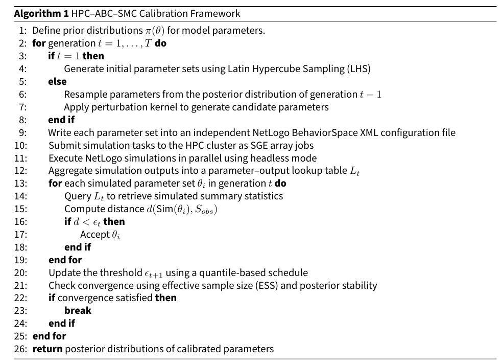
Based on the precomputed result mapping strategy described in sections 3.16–3.19, this study uses an Approximate Bayesian Computation–Sequential Monte Carlo (ABC-SMC) framework to estimate the posterior distribution of model parameters.
ABC-SMC iteratively approximates the posterior distribution through a sequence of particle populations (generations). At each generation, a set of candidate parameter particles is sampled from either the prior distribution (for the first generation) or from the posterior of the previous generation through resampling and perturbation.
For each candidate parameter set, the corresponding simulation outputs are retrieved from the precomputed parameter–output mapping rather than executing the NetLogo model directly. This lookup process replaces repeated interface-based model calls and enables efficient evaluation of large numbers of parameter particles.
Model fit is evaluated by computing the distance between simulated summary statistics and empirical observations. A particle is accepted if the distance falls below a tolerance threshold \(\epsilon\). Across generations, the threshold is gradually reduced using a quantile-based schedule, progressively tightening the acceptance criterion and improving the posterior approximation.
Two independent calibration experiments are conducted in this study: one focusing on the trade partner match rate and the other on the trade volume match rate. Treating these evaluation metrics separately allows each calibration objective to be examined without imposing assumptions about trade-offs between objectives.
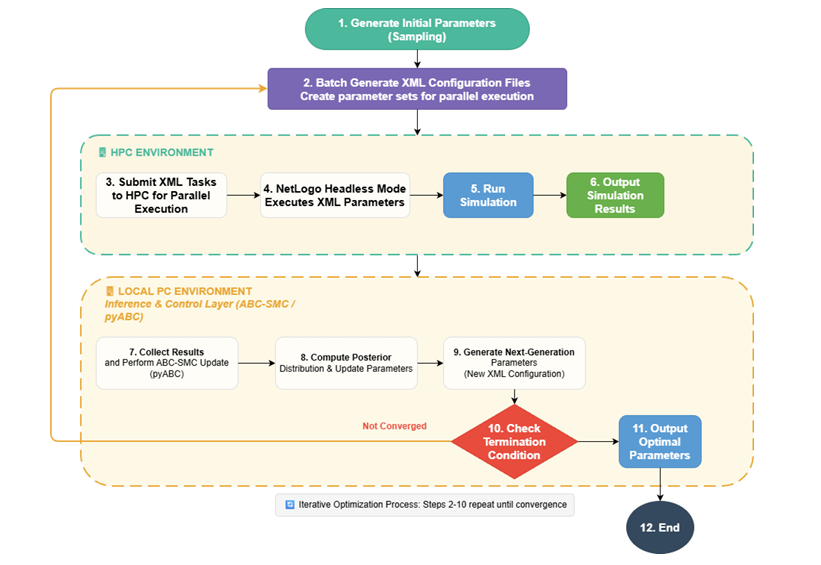
The overall calibration workflow is illustrated in Figure 1. Large-scale
simulation tasks (Steps 3–6) are executed in parallel on the HPC
cluster, while the Bayesian inference process (Steps 7–10) is performed
locally using pyABC. The process iterates across
generations until convergence criteria are met, producing posterior
distributions of the calibrated parameters.
HPC Environment
Computational approach
To support large-scale parameter calibration for the ABM, we employed a task-level parallelization strategy. This approach allowed the full simulation campaign to be completed within a reasonable timeframe while maintaining reproducibility. Each simulation corresponds to a unique parameter combination and is executed as an independent task. Experiment configurations are managed using standard NetLogo BehaviorSpace XML files, where each XML file specifies a distinct parameter combination, enabling systematic experiment management and traceability.
Parallel execution and resource management
Given the limitations of thread-based parallelization in NetLogo, we adopted a task-level parallel execution framework in which each simulation runs independently (Railsback et al. 2017). This design avoids interference between simulations and improves execution stability.
All simulations were submitted to a high-performance computing (HPC) cluster and managed using the Sun Grid Engine (SGE) scheduling system. Tasks were distributed across multiple compute nodes. Each node contains 40 CPU cores and runs up to 10 simulations in parallel, as each simulation instance internally utilizes approximately four CPU threads, including the main execution thread and additional threads for Java garbage collection. This configuration prevents CPU oversubscription and ensures stable memory usage.
To improve scheduling efficiency and fault tolerance, simulation tasks were submitted in batches of 5000. This batching strategy allows failed jobs to be quickly identified and resubmitted without interrupting the overall experiment workflow.
Computational efficiency and reproducibility
The computational framework was designed to ensure scalability and reproducibility. Compared with multi-threaded execution, task-level parallelization reduces CPU contention and improves overall throughput. Because each simulation runs independently, failed tasks can be resubmitted without affecting the rest of the experiment. All experimental configurations are recorded in XML files, ensuring full traceability and facilitating future replication and analysis.
Experimental Results & Analysis
Computational performance evaluation
This study leverages the ARC4 high-performance computing (HPC) cluster at the University of Leeds to execute large batches of NetLogo simulations using the Sun Grid Engine (SGE) job scheduling system. Each simulation corresponds to a unique parameter combination and runs independently. This independence enables efficient distribution of simulations across compute nodes using task-level parallelism.
To illustrate the practical implications of different NetLogo execution strategies commonly used in agent-based modeling workflows, we compare several execution modes, including the default NetLogo GUI mode, pyNetLogo, RNetLogo, and headless NetLogo execution on an HPC cluster. The goal of this comparison is not to provide a strict hardware benchmark, but rather to demonstrate how different execution strategies affect computational efficiency when running repeated simulation experiments.
| Execution Method | Simulations Run | Estimated Time | Speedup vs. Baseline |
|---|---|---|---|
| NetLogo GUI Mode (1 core, PC) | 100 | 800 min (13.3 h) | Baseline (\(1.0 \times\)) |
| pyNetLogo (8 threads, PC) | 100 | \(\sim\)400 min (6.7 h) | \(2.0 \times\) |
| RNetLogo (6 threads, PC) | 100 | \(\sim\)500 min (8.3 h) | \(1.6 \times\) |
| HPC + Headless NetLogo (40 parallel jobs) | 100 | \(\sim\)19 min | \(42.1 \times\) |
| Note: Speedup is calculated relative to the baseline method (NetLogo GUI mode on a single-core PC with view updates enabled). All other execution modes (pyNetLogo, RNetLogo, and HPC with headless NetLogo) were executed without graphical rendering. The HPC configuration runs headless NetLogo simulations as independent tasks scheduled through the ARC4 cluster using the SGE job scheduler. | |||
Table 2 shows that the default NetLogo GUI mode is computationally inefficient for repeated experiments, requiring over 13 hours to complete 100 simulations. By contrast, pyNetLogo and RNetLogo provide moderate improvements by enabling parallel execution through Python and R environments on personal computers. These interfaces typically manage multiple NetLogo instances through external process-based parallelization.
The headless NetLogo configuration combined with task-level parallel execution substantially reduces runtime, completing the same workload in approximately 19 minutes. This result highlights the efficiency of running NetLogo in headless mode together with parallel job scheduling for large-scale simulation experiments. Importantly, the main performance gains arise from eliminating graphical rendering and distributing independent simulation tasks across multiple compute resources, making this approach particularly suitable for computationally intensive calibration workflows.
Benchmark comparison: Random sampling vs. optimization methods
To evaluate the effectiveness of the genetic algorithm (GA) calibration method, we compared the GA approach against a random sampling baseline. To establish a reference benchmark, we generated 30,000 random parameter combinations across the parameter space.The genetic algorithm was implemented with stage-dependent crossover and mutation rates, as summarized in Table 3.
| Stage | Generations | Crossover Rate | Mutation Rate |
|---|---|---|---|
| Initial Phase | 1–5 | 0.7–0.9 | 0.2–0.4 |
| Middle Stage | 6–10 | 0.6–0.7 | 0.3–0.5 |
| Late Stage | 11–20 | 0.4–0.6 | 0.1–0.3 |
Figures 2a and 2b present the fitness evolution for the Trade Partner Matching Rate and Trade Volume Matching Rate during the genetic algorithm optimization. Both figures show that the GA rapidly approaches and slightly exceeds the random sampling baselines (red dashed lines) within the early generations.
In Figure 2a, the Trade Partner Matching Rate exceeds the 68.39% baseline by generation 2 with only 2,000 simulation runs, representing roughly a 15-fold reduction in computational effort compared to random sampling, which required 30,000 simulation runs. Similarly, in Figure 2b, the GA reaches and slightly exceeds the 66.20% volume matching baseline by generation 3 using just 3,000 simulation runs, corresponding to approximately a 10-fold reduction in computational effort. These results highlight GA’s ability to achieve comparable or improved calibration performance using a substantially smaller computational budget.
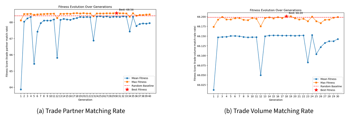
Table 4 summarizes the optimal results of genetic algorithm runs for two distinct calibration objectives: Trade Partner Match Rate and Trade Volume Match Rate. The trade partner objective achieved a maximum fitness of 68.56% in generation 32, whereas the volume objective reached 66.21% in generation 18, indicating faster convergence for the volume calibration objective.
Notably, the optimal parameter values differ substantially between the two runs. For example, weight-trade-initial increased from 1.5142 (partner objective) to 19.6096 (volume objective), while weight-gdp-per-capita increased from 0.0612 to 3.2854. These differences suggest that the two calibration objectives rely on substantially different parameter regimes, highlighting the importance of objective-specific calibration in agent-based models with multiple evaluation criteria.
| Parameter | Trade Partner Match Rate | Trade Volume Match Rate |
|---|---|---|
| Best Generation | 32 | 18 |
| Best Fitness | 68.56% | 66.21% |
| weight-trade-initial | 1.5142 | 19.6096 |
| weight-trade-endo | 0.2315 | 1.3978 |
| weight-gdp-per-capita | 0.0612 | 3.2854 |
ABC-SMC Calibration Outcomes
Our hybrid HPC–ABC-SMC framework was applied to calibrate the agent-based international trade model for two evaluation criteria: Trade Partner Match Rate and Trade Volume Match Rate. The two objectives were calibrated separately using the ABC-SMC procedure. Table 5 presents the final calibrated parameter values with their uncertainty estimates, derived as 95% credible intervals from the posterior distribution of the final ABC-SMC generation (2.5th and 97.5th percentiles of the accepted samples).
| Parameter | Trade Partner Match Rate | Trade Volume Match Rate |
|---|---|---|
| weight-trade-initial | [1.373, 3.330] | [12.847, 19.730] |
| weight-trade-endo | [0.077, 0.556] | [0.116, 3.920] |
| weight-gdp-per-capita | [0.048, 0.418] | [1.369, 4.137] |
Trade Partner Match Rate Optimization
The trade partner match rate optimization converged after 10 generations of ABC-SMC. Figure 5 illustrates the evolution of parameter distributions across generations. The right-side plots include shaded areas representing the standard deviation of parameter values across particles.As shown in Figure 5, all parameters exhibit consistent convergence, with both means stabilizing and variances narrowing significantly in generations 7–9, indicating reduced uncertainty and increasing posterior concentration:
- weight-trade-initial converged from an initial \(12.90 \pm 4.60\) to \(1.73 \pm 0.35\)
- weight-trade-endo decreased from \(9.97 \pm 5.79\) to \(0.30 \pm 0.12\)
- weight-gdp-per-capita reduced from \(8.67 \pm 5.48\) to \(0.13 \pm 0.08\)
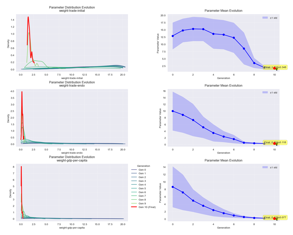
The parameter distributions in the final generation exhibited highly concentrated characteristics, with interquartile ranges of \([1.50, 1.80]\), \([0.21, 0.36]\), and \([0.08, 0.15]\) respectively, indicating strong posterior concentration. Correlation analysis revealed a moderate positive correlation (0.47) between weight-trade-initial and weight-trade-endo, while weight-trade-initial showed a weak negative correlation (-0.23) with weight-gdp-per-capita.
Trade Volume Match Rate Optimization
The trade volume match rate optimization converged within 8 generations of ABC-SMC. Figure 4 illustrates the evolution of parameter distributions across generations. Compared with the trade partner match rate calibration, the parameter trajectories exhibit distinct convergence patterns.
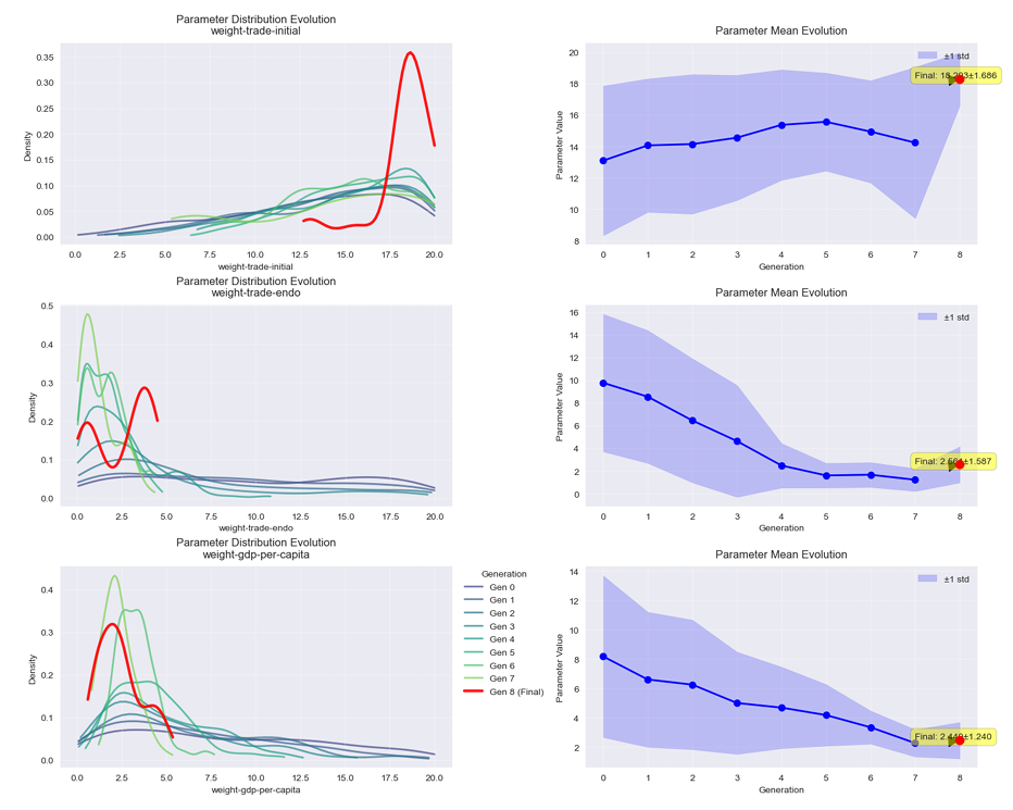
As shown in Figure 4, the parameter evolution demonstrates differentiated behaviour across parameters:
- weight-trade-initial increases steadily, converging from \(13.10 \pm 4.76\) to \(18.29 \pm 1.69\)
- weight-trade-endo decreases from \(9.77 \pm 6.06\) to \(2.56 \pm 1.59\), while retaining some variability
- weight-gdp-per-capita decreases from \(8.17 \pm 5.51\) to \(2.45 \pm 1.24\), showing the strongest convergence pattern
Overall, the parameter distributions stabilise rapidly, with reduced variance across generations, indicating efficient convergence of the ABC-SMC procedure.
Correlation analysis reveals a significant negative correlation (-0.48) between weight-trade-endo and weight-gdp-per-capita, indicating a clear trade-off between these factors in the model.
Validation Against Genetic Algorithm Results
To validate the reliability of our ABC-SMC parameter estimates, we compare the GA optimal parameter combinations with ABC-SMC 95% credible regions across both optimization objectives.
Figure 5 presents the validation results of GA and ABC-SMC in the three-dimensional parameter space, showing strong consistency between the two methods in identifying key parameter regions while also revealing distinct characteristics across the two optimization objectives.
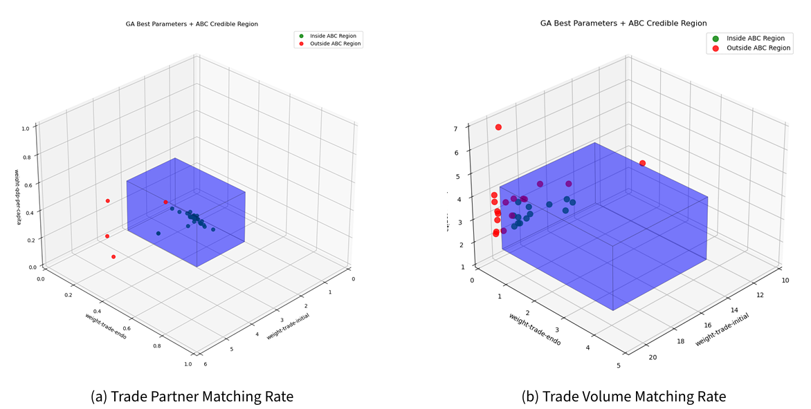
Trade partner match rate validation (Figure 5a): Among the 30 GA-derived optimal parameter sets across generations, 13 sets (43.3%) lie within the 95% credible region produced by ABC-SMC, while the remaining 17 sets are located near the boundary of the region. This distribution pattern, together with the relatively stable trade partner performance across generations, indicates that the trade partner objective is sensitive to parameter changes and that high-performing solutions concentrate in a relatively narrow parameter region.
Trade volume match rate validation (Figure 5b): The results show strong consistency between methods. Only 4 GA solutions fall outside the ABC-SMC credible region, corresponding to a coverage rate of 87%. This suggests that the ABC-SMC framework effectively identifies the parameter space required to achieve optimal trade volume matching. The GA results are tightly clustered within the credible region and mostly located in the low-value parameter range, further confirming that trade volume optimization operates within a well-defined parameter space.
Comparison with Genetic Algorithm Results
To validate the effectiveness of our hybrid HPC-ABC-SMC framework, we also performed parameter calibration using a genetic algorithm (GA) under the same optimization objectives. Table 6 compares the final parameter values obtained by both methods.
| Parameter | ABC-SMC (Partner) | GA (Partner) | ABC-SMC (Volume) | GA (Volume) |
|---|---|---|---|---|
| weight-trade-initial | [1.373, 3.330] | 1.51 | [12.847, 19.730] | 19.61 |
| weight-trade-endo | [0.077, 0.556] | 0.27 | [0.116, 3.920] | 1.40 |
| weight-gdp-per-capita | [0.048, 0.418] | 0.06 | [1.369, 4.137] | 3.29 |
The GA-derived parameters fall within the 95% credible intervals obtained from ABC-SMC, demonstrating strong consistency between the two methods. This consistency supports the robustness of the identified parameter regimes and validates the effectiveness of both approaches.
While GA provides efficient point estimates, ABC-SMC offers a richer calibration outcome by quantifying parameter uncertainty through posterior distributions. This capability is particularly valuable for policy-relevant simulations, where uncertainty ranges can inform sensitivity analysis and robust decision-making. In addition, our HPC-enabled ABC framework achieves high computational efficiency through parallel task execution and the use of precomputed simulation results, making it well suited for computationally intensive agent-based model calibration.
Sensitivity analysis
We conducted a global sensitivity analysis using the Sobol method implemented via the SALib Python library. From Table 7, the sensitivity analysis identifies GDP per capita weight as the most influential parameter, showing the highest total sensitivity indices (\(S_T=0.910\) for trade partner matching and \(S_T=0.939\) for trade volume matching). Endogenous trade weight and initial trade weight follow in consistent rankings across both metrics. All parameters exhibit low first-order indices (\(S_1 \approx 0.1\)) but high total effects, revealing strong nonlinear interactions. This justifies our use of ABC for calibration, as it captures parameter interdependencies missed by conventional methods. The dominance of GDP per capita aligns with gravity model principles, validating economic scale as a core determinant of international trade patterns.
| Trade Partner Rate | Trade Volume Match Rate | ||||||||
|---|---|---|---|---|---|---|---|---|---|
| 2-5 Parameter | \(S1\) | \(S1_{conf}\) | \(ST\) | \(ST_{conf}\) | \(S1\) | \(S1_{conf}\) | \(ST\) | \(ST_{conf}\) | |
| weight-trade-initial | 0.096 | 0.046 | 0.624 | 0.042 | 0.103 | 0.057 | 0.732 | 0.048 | |
| weight-trade-endo | 0.112 | 0.050 | 0.708 | 0.051 | 0.118 | 0.061 | 0.781 | 0.050 | |
| weight-gdp-per-capita | 0.127 | 0.060 | 0.910 | 0.059 | 0.128 | 0.064 | 0.939 | 0.061 | |
| \(S1\): First-order sensitivity index; \(ST\): Total sensitivity index. Confidence values represent the uncertainty range (\(\pm\)) for each sensitivity index | |||||||||
Discussion
The calibration results highlight three mechanisms that drive the evolution of international trade networks:
- Path dependence of trade volumes. In the volume–matching objective, the posterior mean of weight-trade-initial is \(18.29\) (95% CI: \([12.84, 19.73]\))[2], an order of magnitude larger than any other weight. This confirms that historical trade links strongly shape current flow decisions, lending quantitative support to path-dependence arguments in network theory.
- Endogenous partner selection. Under the partner–matching objective, all calibrated weights shrink towards zero (posterior means \(<0.8\) with tight CIs), indicating that partner choice is governed primarily by endogenous search and self-organisation rather than by exogenous attraction factors. This systematic difference in parameter magnitudes between the two objectives reflects their different sensitivities: partner matches are discrete (a correct partner must be selected), whereas volume matches allow partial fits. As a result, the partner-based calibration imposes tighter constraints on parameter values, while the volume-based calibration permits broader ranges.
- Comparison with prior calibrations. Table 8 compares our ABC-SMC posterior means with the benchmark values of Ge et al. (2021). Although the rank ordering of weights is identical, our estimates deviate by 20–45%. Two of the three literature point estimates fall outside our 95% credible interval for the partner match rate, but within the interval for the trade volume objective (see Table 6). For example, the literature value of weight-gdp-per-capita (1.4) lies outside our Partner-based credible interval ([0.048, 0.418]) but within the Volume-based credible interval ([1.369, 4.137]). This divergence reflects both methodological and data differences: the earlier study used UN Comtrade data (42 of 91 categories) and selected a single Pareto-front point from 10,000 LHS samples, while our calibration employs FAO data covering all 97 categories and quantifies uncertainty through ABC-SMC. Our results therefore extend prior work by showing how point estimates may fall within one calibration target but outside another, highlighting the value of uncertainty-aware calibration.
| Parameter | Our Study (Partner, mean) | Our Study (Volume, mean) | Literature Value* |
|---|---|---|---|
| weight-trade-initial | 1.73 | 18.29 | 1.40 |
| weight-trade-endo | 0.30 | 2.56 | 0.72 |
| weight-gdp-per-capita | 0.13 | 2.45 | 1.40 |
| *Reference values: GDP = 1.40, Distance = 1 (fixed), Historic trade = 1.40, Emergent trade = 0.72. | |||
| Note: Values reported for Our Study are posterior means from ABC-SMC calibration. Differences from the literature partly reflect dataset coverage (97 categories in our FAO trade data vs. 42 in the original Comtrade-based study). | |||
Overall, these results demonstrate the practical applicability of the proposed calibration framework and provide additional insights into potential mechanisms underlying international trade network formation. In particular, we find that trade partner relationship formation and trade volume determination may be driven by different mechanisms, which may help inform the development of trade models.
Moreover, by calibrating the two objectives separately rather than through a simultaneous multi-objective framework, we can show more clearly how different evaluation criteria constrain parameters in distinct ways, avoiding unfair trade-offs and clarifying parameter sensitivities under each objective. The use of ABC-SMC also enables posterior uncertainty to be quantified, providing a richer interpretation of parameter ranges.
Finally, compared to earlier calibrations, our updated dataset and more disaggregated commodity categories reveal systematic shifts in parameter magnitudes, underscoring how empirical refinements can reshape the balance between partner-driven and volume-driven mechanisms in international trade.
Conclusion
This study introduces a precomputed result mapping strategy, the central methodological contribution of this work, that decouples agent-based model simulation from statistical inference. By batch-executing NetLogo simulations as independent HPC tasks and organising their outputs into parameter–output lookup tables, the framework enables ABC-SMC inference to proceed by querying stored results rather than repeatedly invoking the simulator through interface-based tools such as PyNetLogo or RNetLogo. Applied to a global food trade model, this design achieves a 42-fold reduction in wall-clock time relative to GUI-based single-core execution, while preserving the full statistical rigour of the calibration procedure.
Unlike conventional optimisation approaches that yield only single best-fit parameter sets, the HPC-ABC-SMC framework produces full posterior distributions with 95% credible intervals, enabling richer interpretation of parameter uncertainty. Cross-validation with genetic algorithm results confirms the robustness of the posterior estimates: the single best-fit GA solution for each objective falls within the corresponding ABC-SMC 95% credible interval.
The calibration results reveal systematic differences between the two objectives: trade partner calibration converges to small parameter magnitudes within narrow credible intervals, reflecting high sensitivity to parameter perturbations, whereas trade volume calibration requires substantially larger weights for historical trade relationships, consistent with path-dependence mechanisms in international trade networks.Sensitivity analysis further identifies GDP per capita weight as the most influential parameter, with strong nonlinear interactions across all three calibrated weights.
Several limitations should be noted. The current implementation assigns one simulation per parameter combination without explicitly modelling stochastic variability across random seeds; incorporating multiple realisations per parameter point would strengthen the robustness of the precomputed mapping. Future work will also explore automatic convergence criteria, surrogate-assisted acceleration, and neural simulation-based inference as a complementary approach (Dyer et al. 2024; Platt 2022), as well as extension to ABMs with higher-dimensional parameter spaces and joint multi-objective calibration.
Overall, the precomputed result mapping strategy offers a generalisable architectural pattern for any simulation platform that supports batch execution, providing a scalable and uncertainty-aware pathway for Bayesian calibration of computationally intensive agent-based models.
Code availability
The code repository is available at: https://github.com/Kejian2023/ABC-SMC-Framework.Acknowledgements
The authors thank the editor and reviewers for their constructive comments, which helped improve the clarity and presentation of this article. We also acknowledge the University of Leeds and The James Hutton Institute for providing research support, HPC training, and computational resources that made this work possible.The authors gratefully acknowledge the guidance, support, and intellectual contribution of the late Dr Jiaqi Ge, our co-author. This article is dedicated to her memory. Her untimely passing is a great loss to us and to the wider academic community.
Appendix
Appendix A: <Summary-ODD>
This model builds on the relation-driven global food trade model originally developed by (Ge et al. 2021). For ODD components that remain unchanged, readers are referred to the original description. The present version introduces three main updates: (i) the calibration and validation database has been extended to cover the years 2010–2022, (ii) the FAO datasets have been updated, including trade, food balance sheets, population, and GDP, and history trade data. (iii) The number of food categories has been expanded from 91 to 97. These modifications are reflected in the Input Data section below.
Purpose
The relation-driven agent-based global trade model is designed to investigate how four key factors—GDP per capita, geographic distance, historic trade relationships, and emergent trade relationships—influence bilateral food trade flows and their implications for national food and nutrition security. Rather than relying on price or comparative advantage, the model lets each country rank potential trade partners based on these structural and relational factors and select partners accordingly. It provides a flexible platform to explore global scenarios such as climate change, sustainable intensification, waste reduction, and dietary transitions.
Entities, State Variables, and Scales
Entities: The model includes all world countries, each represented as an agent.
State variables: Each country is defined by its population, GDP, food production (by commodity group), bilateral trade matrix, strength of historical and evolving trade relations, dietary structure, and food loss rate.
Spatial scale: Countries are assigned geographic locations based on global shapefiles; the model is spatially explicit.
Temporal scale: One simulation step represents one year. The simulation spans from 2010 to 2050.
Process Overview and Scheduling
Each simulation year follows a sequential structure:
Update exogenous country-level attributes: population, GDP, and food production.
Assess national demand–supply balance to determine trade needs.
Rank potential trade partners based on a composite score integrating GDP per capita, geographic distance, historical trade volume, and emerging trade ties.
Execute bilateral trade via a partner-matching algorithm.
Design Concepts
Emergence: Trade structures and evolving trade networks emerge from decentralized bilateral decision-making.
Interaction: Countries interact through an iterative trade matching process based on multi-criteria partner rankings.
Stochasticity: The order of partner matching is randomized each year; simulation outputs are averaged across runs.
Initialization
The model is initialized using average values from the 2010–2012 FAOSTAT Food Balance Sheets and bilateral trade matrices. Initial trade ties reflect historical volumes and are updated dynamically throughout the simulation.
Input Data
The original model (Ge et al. 2021) employed FAO trade and food balance sheet data for 2001–2007 (calibration) and 2008–2013 (validation). For the trade partner index, it relied on UN Comtrade data, which only covered 42 of the 91 food categories in FAO.
In this study, the database has been updated and extended to cover 2010–2022. Population and GDP data are sourced from FAO, with forward projections based on SSPs. Food production and trade flows are derived from FAO, using the most recent bilateral trade matrices and food balance sheets. Importantly, we reconstructed the partner index using FAO trade data directly, allowing coverage of all food categories, and refined the food categorisation by increasing the number of items from 91 in the original model to 97 in this study.
Sub-models
Trade ranking module: Calculates composite scores for trade partner selection using weighted criteria (GDP per capita, geographic distance, historical trade, emergent ties).
Trade execution module: Matches importer demand with exporter supply, subject to partner ranking and capacity limits.
Endogenous update module: Reinforces bilateral ties through feedback from realized trade flows.
Appendix B: <Evolution of Model Parameters in ABC-SMC>
| Generation | weight-trade-initial | weight-trade-endo | weight-gdp-per-capita |
| Mean ± Std | Mean ± Std | Mean ± Std | |
| 0 | 12.8963 ± 4.6004 | 9.9730 ± 5.7947 | 8.6669 ± 5.4755 |
| 1 | 14.7859 ± 4.0581 | 8.8679 ± 5.3341 | 7.1786 ± 4.7694 |
| 2 | 15.2905 ± 4.1552 | 7.3045 ± 4.7929 | 4.9497 ± 3.0280 |
| 3 | 15.2141 ± 4.0819 | 5.1308 ± 3.1952 | 3.5601 ± 2.2493 |
| 4 | 13.5946 ± 5.0965 | 3.4597 ± 2.5325 | 2.4117 ± 1.6651 |
| 5 | 13.3164 ± 5.0147 | 2.3575 ± 1.6384 | 1.5800 ± 1.0764 |
| 6 | 12.2505 ± 5.1755 | 1.6025 ± 1.2229 | 0.9451 ± 0.5966 |
| 7 | 8.5535 ± 5.4691 | 0.5121 ± 0.3299 | 0.5239 ± 0.3001 |
| 8 | 3.5462 ± 1.7090 | 0.3684 ± 0.2005 | 0.3002 ± 0.1811 |
| 9 | 1.9518 ± 0.5283 | 0.2732 ± 0.1385 | 0.2056 ± 0.1249 |
| 10 | 1.7329 ± 0.3477 | 0.3039 ± 0.1178 | 0.1287 ± 0.0772 |
| Generation | weight-trade-initial | weight-trade-endo | weight-gdp-per-capita |
| Mean ± Std | Mean ± Std | Mean ± Std | |
| 0 | 13.0975 ± 4.7588 | 9.7683 ± 6.0589 | 8.1715 ± 5.5124 |
| 1 | 14.0675 ± 4.2445 | 8.5420 ± 5.8520 | 6.6014 ± 4.6046 |
| 2 | 14.1481 ± 4.4386 | 6.4449 ± 5.4608 | 6.2528 ± 4.4171 |
| 3 | 14.5555 ± 3.9838 | 4.6345 ± 4.9295 | 5.0006 ± 3.4868 |
| 4 | 15.3732 ± 3.5129 | 2.4788 ± 1.9611 | 4.6842 ± 2.7785 |
| 5 | 15.5650 ± 3.1168 | 1.6057 ± 1.0832 | 4.1750 ± 2.0971 |
| 6 | 14.9421 ± 3.2535 | 1.6648 ± 1.0911 | 3.3410 ± 1.1269 |
| 7 | 14.2381 ± 4.8125 | 1.2215 ± 1.0021 | 2.2642 ± 0.9224 |
| 8 | 18.2928 ± 1.6861 | 2.5608 ± 1.5873 | 2.4489 ± 1.2395 |
Appendix C: <ABC–SMC Calibration Workflow>
For clarity and reproducibility, the calibration procedure implemented in this study is summarised in Algorithm 1. The algorithm describes how parameter sets are iteratively generated, evaluated through HPC-based NetLogo simulations, and accepted or rejected within the ABC–SMC framework using a precomputed parameter–output mapping.
Notes
- Source: https://github.com/quaquel/pyNetLogo/issues/79.↩︎
- All credible intervals are based on 105 ABC–SMC draws.↩︎
References
Axtell, R. L., & Farmer, J. D. (2025). Agent-based modeling in economics and finance: Past, present, and future. Journal of Economic Literature, 63(1), 197–287. [doi:10.1257/jel.20221319]
Beaumont, M. A. (2019). Approximate Bayesian computation. Annual Review of Statistics and Its Application, 6, 379–403. https://doi.org/10.1146/annurev-statistics-030718-105212 [doi:10.1146/annurev-statistics-030718-105212]
Bianchi, F., & Squazzoni, F. (2015). Agent-based models in sociology. Wiley Interdisciplinary Reviews: Computational Statistics, 7(4), 284–306. [doi:10.1002/wics.1356]
Carrella, E. (2021). No free lunch when estimating simulation parameters. Journal of Artificial Societies and Social Simulation, 24(2). [doi:10.18564/jasss.4572]
Dyer, J., Cannon, P., Farmer, J. D., & Schmon, S. M. (2024). Black-box bayesian inference for agent-based models. Journal of Economic Dynamics and Control, 161, 104827. [doi:10.1016/j.jedc.2024.104827]
Ekström, H., Droste, N., & Brady, M. (2024). Modelling forests as social-ecological systems: A systematic comparison of agent-based approaches. Environmental Modelling & Software, 175, 105998. [doi:10.1016/j.envsoft.2024.105998]
Ge, J., Polhill, J. G., Macdiarmid, J. I., Fitton, N., Smith, P., Clark, H., Dawson, T., & Aphale, M. (2021). Food and nutrition security under global trade: A relation-driven agent-based global trade model. Royal Society Open Science, 8(1), 201587. [doi:10.1098/rsos.201587]
Gilbert, N., Ahrweiler, P., Barbrook-Johnson, P., Narasimhan, K. P., & Wilkinson, H. (2018). Computational modelling of public policy: Reflections on practice. Journal of Artificial Societies and Social Simulation, 21(1). [doi:10.18564/jasss.3669]
Grazzini, J., Richiardi, M. G., & Tsionas, M. (2017). Bayesian estimation of agent-based models. Journal of Economic Dynamics and Control, 77, 26–47. [doi:10.1016/j.jedc.2017.01.014]
Grimm, V., Revilla, E., Berger, U., Jeltsch, F., Mooij, W. M., Railsback, S. F., Thulke, H.-H., Weiner, J., Wiegand, T., & DeAngelis, D. L. (2005). Pattern-oriented modeling of agent-based complex systems: Lessons from ecology. Science, 310(5750), 987–991. [doi:10.1126/science.1116681]
Gunaratne, C., & Garibay, I. (2021). NL4Py: Agent-based modeling in python with parallelizable NetLogo workspaces. SoftwareX, 16, 100801. [doi:10.1016/j.softx.2021.100801]
Jaxa-Rozen, M., & Kwakkel, J. H. (2018). Pynetlogo: Linking netlogo with python. Journal of Artificial Societies and Social Simulation, 21(2). [doi:10.18564/jasss.3668]
Klinger, E., Rickert, D., & Hasenauer, J. (2018). pyABC: Distributed, likelihood-free inference. Bioinformatics, 34(20), 3591–3593. [doi:10.1093/bioinformatics/bty361]
Lamperti, F., Roventini, A., & Sani, A. (2018). Agent-based model calibration using machine learning surrogates. Journal of Economic Dynamics and Control, 90, 366–389. [doi:10.1016/j.jedc.2018.03.011]
Lee, J.-S., Filatova, T., Ligmann-Zielinska, A., Hassani-Mahmooei, B., Stonedahl, F., Lorscheid, I., Voinov, A., Polhill, J. G., Sun, Z., & Parker, D. C. (2015). The complexities of agent-based modeling output analysis. Journal of Artificial Societies and Social Simulation, 18(4). [doi:10.18564/jasss.2897]
Lippe, M., Bithell, M., Gotts, N., Natalini, D., Barbrook-Johnson, P., Giupponi, C., Hallier, M., Hofstede, G. J., Le Page, C., Matthews, R. B., et al. (2019). Using agent-based modelling to simulate social-ecological systems across scales. GeoInformatica, 23(2), 269–298. [doi:10.1007/s10707-018-00337-8]
McKay, M. D., Beckman, R. J., & Conover, W. J. (2000). A comparison of three methods for selecting values of input variables in the analysis of output from a computer code. Technometrics, 42(1), 55–61. [doi:10.1080/00401706.2000.10485979]
Platt, D. (2020). A comparison of economic agent-based model calibration methods. Journal of Economic Dynamics and Control, 113, 103859. [doi:10.1016/j.jedc.2020.103859]
Platt, D. (2022). Bayesian estimation of economic simulation models using neural networks. Computational Economics, 59(2), 599–650. [doi:10.1007/s10614-021-10095-9]
Railsback, S., Ayllón, D., Berger, U., Grimm, V., Lytinen, S., Sheppard, C., & Thiele, J. C. (2017). Improving execution speed of models implemented in NetLogo. [doi:10.18564/jasss.3282]
Salecker, J., Sciaini, M., Meyer, K. M., & Wiegand, K. (2019). The nlrx r package: A next-generation framework for reproducible NetLogo model analyses. Methods in Ecology and Evolution, 10(11), 1854–1863. [doi:10.1111/2041-210x.13286]
Sun, Z., Lorscheid, I., Millington, J. D., Lauf, S., Magliocca, N. R., Groeneveld, J., Balbi, S., Nolzen, H., Müller, B., Schulze, J., et al. (2016). Simple or complicated agent-based models? A complicated issue. Environmental Modelling & Software, 86, 56–67. [doi:10.1016/j.envsoft.2016.09.006]
Thiele, J. C., Kurth, W., & Grimm, V. (2012). RNetLogo: An r package for running and exploring individual-based models implemented in NetLogo. Methods in Ecology and Evolution, 3(3), 480–483. [doi:10.1111/j.2041-210x.2011.00180.x]
Toni, T., Welch, D., Strelkowa, N., Ipsen, A., & Stumpf, M. P. (2009). Approximate bayesian computation scheme for parameter inference and model selection in dynamical systems. Journal of the Royal Society Interface, 6(31), 187–202. [doi:10.1098/rsif.2008.0172]
Vaart, E. van der, Beaumont, M. A., Johnston, A. S., & Sibly, R. M. (2015). Calibration and evaluation of individual-based models using approximate bayesian computation. Ecological Modelling, 312, 182–190.
Verhagen, H., Moss, S., Gilbert, N., Paolucci, M., Andrighetto, G., Jager, W., Ernst, A., Squazzoni, F., Polhill, G., & Ahrweiler, P. (2021). Past, present, and future of agent-based social simulation modelling—presidential views. Conference of the European Social Simulation Association, 517–536. [doi:10.1007/978-3-031-91782-0_38]
Wang, X., Jenner, A. L., Salomone, R., Warne, D. J., & Drovandi, C. (2024). Calibration of agent based models for monophasic and biphasic tumour growth using approximate bayesian computation. Journal of Mathematical Biology, 88(3), 28. [doi:10.1101/2022.09.13.507714]
Wilensky, U. (2023). NetLogo 6.4.0 user manual. https://ccl.northwestern.edu/netlogo/docs/NetLogo%20User%20Manual.pdf
Windrum, P., Fagiolo, G., & Moneta, A. (2007). Empirical validation of agent-based models: Alternatives and prospects. Journal of Artificial Societies and Social Simulation, 10(2), 8.