Mapping Complex Agent-Based Model Parameter Spaces Using Metamodels and Mixed Adaptive Sampling

,
and
University of Texas at Arlington, United States
Journal of Artificial
Societies and Social Simulation 29 (3) 6
<https://www.jasss.org/29/3/6.html>
DOI: 10.18564/jasss.6161
Received: 04-Aug-2025 Accepted: 28-Jun-2026 Published: 30-Jun-2026
Abstract
Large-scale agent-based models (ABM) of complex adaptive systems often have a high number of input parameters and complicated agent interactions affecting the performance of the system. Executing traditional design of experiments to select points from the parameter space could require considerable simulation runs to effectively analyze the impact of input parameters on the system output. Sequential sampling is a promising technique for reducing simulation runs by training a machine learning metamodel to emulate the relationship between input parameters and ABM outputs while leveraging the metamodel to strategically select points to explore next in the parameter space. While previous studies have applied sequential sampling to few small ABMs, this research extends the approach to large-scale ABM and compares mixed adaptive sampling and pure sequential sampling algorithms. These algorithms were used to train a random forest metamodel emulating the Segregation model and a larger stylized ABM of a crowd logistics platform. Results indicate that the pure sequential sampling algorithm can lead to excessive clustering of design points in highly nonlinear regions and insufficient exploration of the parameter space, while the mixed adaptive sampling algorithm ensures broader coverage of the parameter space while still refining complex regions. The mixed adaptive sampling algorithm was then used to generate feature importance and partial dependence plots for the crowd logistics ABM, thereby demonstrating the usefulness of this approach not only in reducing computational requirements for ABM experimentation but also in enhancing ABM output interpretation.Introduction
Agent-based modeling (ABM) is a valuable tool for studying emergent system-level behavior of complex adaptive systems by modeling the behavior of autonomous individual agents that are capable of responding and adapting to inputs from their environment (Dooley 1996; Marchi & Page 2014). In complex systems, the repeated interactions among heterogeneous actors over time can lead to global emergent properties, which can be observed by exploring the model’s parameter space (Holland 1992; Srbljinović & Škunca 2003). By modeling these interactions, ABM is capable of producing rich multidimensional system and agent-level data that can serve as important measures of system performance (Lee et al. 2015) and provide researchers and policymakers with a better understanding of how different factors affect agent behavior and resulting emergent system-level behavior. These outputs can then support the development of effective strategies or policy interventions to improve system design, performance, and outcomes (Holland 1992; R. Liu 2022).
However, as the number of different agents and the complexity of their behavioral logic increase, so does the number of parameters and the overall complexity of the model. For example, models of evolution, epidemiology, and biological systems can have more than 200 parameters available for experimentation (Garg et al. 2019), making it computationally expensive to explore the entire parameter space (R. Vahdati et al. 2019). ABM also lacks established methods for interpreting large amounts of model-generated output data (Broeke et al. 2016; James et al. 2021; Saltelli et al. 2019), which has limited its ability to meaningfully inform real-life system design or policy interventions. Moreover, specific guidance on efficient and effective presentation and analysis of ABM outputs is lacking (Lee et al. 2015; Platas-López et al. 2023).
The analysis of simulation output can be facilitated by the use of controlled experimentation with statistical modeling or machine learning (V. C. P. Chen et al. 2006). The resulting approximation models, known as metamodels, allow for rapid generation of approximated simulation output without running the time-consuming simulation (Pereda et al. 2017). Metamodels have long been established as a promising and reliable method to analyze simulation output (L. W. Friedman & Pressman 1988). Indeed, a review of applications of machine learning (ML) methods to ABM found that approximating the relationship between model inputs and outputs using ML techniques can reduce computational costs (Platas-López et al. 2023). Common techniques for developing metamodels include classification and regression trees, random forest, support vector machines, and artificial neural networks. Methods like neural networks are considered “black box” approaches, due to their complex structures and lack of interpretability, while other methods (e.g., random forest) provide better transparency and insights into model behavior by providing metrics on relative variable importance (Musolf et al. 2022). However, creating a reliable ML metamodel for a large and complex ABM might require thousands of runs to sufficiently capture the variability across the input parameter space if an efficient sampling strategy (i.e., choice of simulation input parameter combinations) is not used (Barton 2020; Janssen et al. 2019).
To reduce the number of simulation runs while ensuring that the required accuracy is achieved, metamodels can be used to guide the sampling approach, as with adaptive or sequential sampling (Crombecq et al. 2009). With sequential sampling, candidate design points are iteratively generated and evaluated to test the metamodel’s ability to predict simulation outputs accurately. A high variance in the predictions at a candidate design point indicates that the metamodel needs more information in that region to capture a complex nonlinear input-output relationship. Therefore, the points with highest variance in predictions are chosen next to run the simulation, then retrain the metamodel, until the metamodel achieves a desired accuracy (H. Liu et al. 2018). Indeed, (Edali & Yücel 2019) applied sequential sampling to experimentation with two parameters of the well-known Segregation ABM, allowing them to build a metamodel that suitably characterized ABM outputs over the parameter space while also reducing the number of required runs. While these results were encouraging, the authors pointed out the need for this approach to be tested on a larger ABM with more input parameters.
To address this need, the research described in this paper evaluates pure sequential sampling and mixed adaptive sampling methods to develop metamodels of a relatively small ABM (Segregation model) having two input parameters and a larger ABM (crowd logistics model) with ten input parameters. Furthermore, various configurations of these sampling algorithms were evaluated to guide agent-based modelers in exploring metamodeling approaches to improve experimental efficiency and understand the extent to which each input parameter influences output metrics. The paper reviews the literature on analysis of complex ABMs using metamodeling and then describes the sequential and mixed adaptive sampling algorithms in detail. Experimentation and results with both ABMs are described, including insights into the relationships that were revealed between model parameters and platform performance metrics, followed by a conclusion and recommendations for future research.
Literature Review
This section reviews the literature on ABM output analysis, including traditional design of experiments, metamodeling using machine learning, and sequential sampling to efficiently explore the ABM parameter space.
Experimental designs for output analysis
ABMs produce multi-dimensional data resulting from repeated micro-level agent behavior and interactions over time. Increases in available computational power have allowed for the development of increasingly complex models. However, increasing model size and complexity has led to greater challenges in assessing the sensitivity of a model to varying experimental conditions (Lee et al. 2015). To reduce computational burden and facilitate interpretation of relationships between input parameters and output metrics of interest, a variety of different statistical approaches can be employed. Design of experiments is a systematic approach to designing a statistically valid experiment that obtains maximum useful information about the variation in the output metrics and their relation to the input parameters without requiring a complete parameter sweep (Dean & Voss 1999; Kasaie & Kelton 2015). For example, (Alam et al. 2015) used an orthogonal array design to study the impact of 25 input parameters at four levels in an ABM that simulated immune system response to Heliobacter pylori infection. Similarly, (Hussain & Ali 2019) used orthogonal arrays to experiment with an ABM of a flexible manufacturing system with three factors of interest at three levels. However, construction of these experimental designs requires fixed levels for each factor, which restricts the choice of levels in a factor and can increase the number of experimental runs required to maintain orthogonality (Bose & Bush 1952; Sloane 2012).
One way to mitigate these limitations is to use space-filling experimental designs. The number-theoretic method can be used to generate low-discrepancy sequences that result in space-filling designs with consistent and evenly spread-out design points, unlike purely random sequences, which tend to cluster in some areas and leave gaps in others (Fang & Wang 1993). Among these, Sobol’ sequence is widely used, as it generally performs better in higher dimensional space by covering the parameter space more evenly than other designs, such as Halton and Hammersley (Atanassov et al. 2021; Azmin & Stobart 2015; Burhenne et al. 2011; Sobol 1967). Low discrepancy sequences like Sobol’ enable a thorough exploration of the parameter space in a simulation, which is crucial for accurately understanding the influence of input parameters on model outputs (Sobol′ 2001).
Saltelli sampling extends Sobol’s method by tailoring the sequence to facilitate variance-based global sensitivity analysis, which systematically quantifies the influence of input parameters on the variability of model outputs in a simulation (Saltelli et al. 2008). (Venugopalan et al. 2023) used Saltelli sampling to perform sensitivity analysis on an ABM that simulated an epidemic within a small community. Their objective was to determine which of four state transition probabilities (e.g., transitions from susceptible to exposed, or exposed to infected) had the most significant impact on the spread of the disease by running 320 experiments with 5 replications. However, Saltelli sampling is computationally expensive for a larger number of input parameters, because all Sobol' sample points must be labeled, meaning every design point must have a corresponding output value, which can only be determined by running the ABM.
An alternative method that has been used for ABM output analysis is causal discovery. Causal discovery helps interpret the influence of inputs on outputs by identifying cause-and-effect relationships among variables using observed data. This is often achieved through algorithms that infer causality and represent the relationships as directed acyclic graphs (Huber 2024). However, evaluating a model with many input parameters can complicate the structure of the causal relations, making interpretation and validation more challenging (Chang et al. 2023; Cheng et al. 2024).
Metamodeling
The challenges discussed in the previous section on output analysis can be mitigated by developing metamodels. A metamodel serves as a simplified representation of an ABM, capturing the complex nonlinear relationships between the model’s input parameters and output data. It emulates the ABM, enabling rapid predictions for new input configurations without the need for full-scale simulations.
Machine learning (ML) is a broad field of algorithms that adaptively learn patterns from data and work effectively with complex, nonlinear, or unstructured datasets (Rasmussen 2004). ML approaches have been widely applied to all phases of ABM development, including design and validation, as well as output analysis (Platas-López et al. 2023). In their research comparing the performance of various ML metamodels based on their mean squared error (MSE), (Angione et al. 2022) trained the models on 200, 400, 800, and 1600 ABM runs with 10 input parameters. Across the independent simulation runs, they found that the neural networks ML model consistently achieved the highest prediction accuracy, although it required significantly longer training times compared to other methods. (Larie et al. 2021) and (S. H. Chen et al. 2021) have developed neural network metamodels of ABMs simulating the progression of sepsis and spread of bacteria, respectively. However, the models could not be used to assess the influence of input parameters on the output due to the lack of interpretability of neural networks (Frasca et al. 2024). ML algorithms such as k-means clustering algorithms have also been used for ABM output analysis (Li et al. 2022); however, challenges include random initialization of centroids, susceptibility to outliers, and inefficiency in high-dimensional data due to the curse of dimensionality (Ahmed et al. 2020). Similarly, using support vector machines presents challenges, such as managing high-dimensional and noisy data, selecting appropriate kernel functions, and interpreting the models, because the complex decision boundaries (i.e., surfaces that separate different classes in the feature space) make it difficult to directly link input variables to the output (Cervantes et al. 2020).
Another ML method used for metamodeling is decision trees, which make predictions by recursively splitting input data into subsets based on their value, using criteria like information gain or Gini impurity to determine optimal splits (Quinlan 1986). (Bhattacharjee et al. 2019) used decision trees to explore and explain the decision-making behaviors of agents in an ABM that simulated the communication of fear and safety signals among animals in a foraging context. While decision trees are interpretable, their simplicity can limit their ability to capture the complex interactions in dynamic systems like ABMs (Breiman et al. 2017). Ensemble methods address this issue by combining multiple decision trees and employing techniques such as bagging (e.g., random forests) (Breiman 2001) and gradient boosting to improve the accuracy and robustness of the resulting metamodel. Gradient boosted trees (e.g., XGBoost) is a specific type of boosting where decision trees are built sequentially, with each decision tree correcting the errors of the previous one by optimizing a loss function (J. H. Friedman 2001). These techniques can efficiently handle high-dimensional input spaces, enabling the identification of key drivers of system behavior and offering more precise insights into how input parameters influence outcomes, making them a good choice for developing ABM metamodels (Breiman 2001; T. Chen & Guestrin 2016). Furthermore, (Papacharalampous et al. 2023) and (Shao et al. 2024) found that boosted trees generally outperform random forest, in terms of prediction accuracy.
To efficiently utilize computational resources while enhancing the metamodel's prediction accuracy, sequential or adaptive sampling techniques can be employed to choose which sample points should be used for running the simulation (Crombecq et al. 2011). These techniques focus on highly nonlinear parts of the parameter space, since these regions are more likely to exhibit complex behavior that significantly impact the model's performance and accuracy (Crombecq et al. 2009). (Edali & Yücel 2019) demonstrated the use of sequential sampling with a random forest ML model to refine a metamodel of two well-known ABMs: the Segregation model (Schelling 1971) and the Traffic model (Nagel & Schreckenberg 1992). They used the variance in the predictions of the individual decision trees to help select new sample points to iteratively retrain the metamodel. In this process, all the new points selected were in the regions where the nonlinearity was highest, leaving other regions unexplored.
Indeed, in sequential sampling, exploiting patterns in the current metamodel risks focusing excessively on regions where the response surface is already sufficiently modeled and potentially overlooking other critical regions . This issue can be mitigated by adopting a sequential sampling framework proposed by (Ozik et al. 2018), who developed a metamodel of an ABM simulating the spread of an infectious disease. In each iteration, five new points were selected using the metamodel, while five additional points were randomly sampled, seeking a balance between exploitation and exploration. However, a potential limitation is the selection of five points via exploitation using the same current metamodel, which means they are all based on the same information. While selecting multiple points for exploitation might seem appropriate to speed up the algorithm, only the first point is maximizing the exploitation aspect, and the remaining four are suboptimal and likely redundant. Leveraging exploitation requires obtaining the information on the response surface from that first point before deciding on the next point. Therefore, selecting just one point per iteration can help maximize information gain and avoid redundancy, as (Cohn et al. 1994) suggest for improving generalization, while (H. Liu et al. 2018) note that it can be simpler and more effective.
Further, instead of random sampling, exploration can also be improved using the mixed adaptive sampling approach proposed by (Eason & Cremaschi 2014). The selection of a new point is not only based on the variance in the metamodel’s predictions (i.e., exploitation), but also on the distance of the new points from the existing points that have been used to train the metamodel (i.e., exploration), thereby enabling exploration of the parameter space. The authors demonstrated the effectiveness of this approach by applying it to the Ackley function in MATLAB. Pure adaptive sampling or sequential sampling was unable to model the response surface accurately, while the mixed adaptive sampling approach effectively captured the nonlinearities of the Ackley function (Eason & Cremaschi 2014).
Research contribution
The overarching question that this research seeks to address is: What is the best approach to developing an ML metamodel to serve as an ABM surrogate, in terms of computational efficiency, prediction accuracy, and interpretability? Previous research demonstrated that using sequential sampling to build ML metamodels of small-scale ABMs (i.e., Segregation and Traffic) is an effective approach, enabling strategic selection of design points with which to run the simulation (Edali & Yücel 2019). However, this approach has not been tested on an ABM with more than two input parameters, wherein it could be quite valuable in reducing the number of required simulation runs and facilitating output analysis and interpretation of model behavior. Furthermore, the performance of different sampling algorithm configurations has not been fully explored.
The research described in this paper seeks to address these gaps by comparing the performance of a sequential sampling algorithm that purely exploits (SSA) with the performance of a mixed adaptive sampling algorithm (MASA) in developing tree based random forest ML metamodels of two ABMs: the Segregation model (a small model with two input parameters) and a stylized model of a crowd logistics system (a larger model with 10 input parameters). Tree-based algorithms, as discussed earlier, offer a balance between accuracy, efficiency, robustness, and interpretability, making them an excellent choice for creating metamodels of ABMs for output analysis. The Segregation ABM was chosen to serve as a baseline model for comparison, while the crowd logistics ABM was chosen for practical reasons: prior experimentation with this model had faced significant challenges with respect to computational intensity and output interpretation, limiting its usefulness in research. With 10 input parameters having 5 experimental levels, a full factorial experiment with only single replications would require \(5^{10} = \ 9,765,625\) runs, where each run requires up to 20 minutes. It was hoped that metamodeling could be employed to reduce this computational burden while also providing meaningful insights into the relationships between model inputs and outputs.
Research Methodology
This section describes the implementation of the pure sequential sampling algorithm (SSA) and the mixed adaptive sampling algorithm (MASA).
Pure sequential sampling
With the pure exploitive sequential sampling algorithm (SSA), an initial set of space filling points is generated using an experimental design, such as Latin Hypercube or Sobol sequence. These points are then divided into training (\(S\)) and test data sets (\(T\)), where the simulation is first run for all test points with at least 30 replications per point. The responses of these 30 replications per design point are averaged to generate one target output per point. Once the test data has been acquired, a few points are chosen from the training set to run the simulation (responses are again averaged over the number of replications). Any design point in the training set for which simulation has been run is called a labeled design point and the remaining points are unlabeled. This completes the setup process such that the algorithm can begin its first iteration.
The labeled data from the training set are used to train an initial metamodel (e.g., random forest), which can then evaluate the prediction uncertainty at the unlabeled design points. Prediction uncertainty is calculated using the standard deviation among the predictions made by the decision trees in the random forest metamodel. In each iteration of the algorithm, the unlabeled design point with the highest prediction uncertainty is chosen to run the simulation. The new data point is then added to the labeled dataset, and the model is retrained on it. This process repeats until the computational budget is exhausted. The algorithm uses the test data set to monitor metamodel performance, which is evaluated using coefficient of Determination (\(R^{2}\)), defined as \(R^{2} = 1 - \frac{SSE}{SST}\), where SSE is the sum of squared errors and SST is total sum of squares. The \(R^{2}\) value may also be used as a stopping criterion for the sequential sampling process. For an example of a detailed implementation of this algorithm to analyze an ABM, refer to Edali and Yücel (2019).
Mixed adaptive sampling
The pseudocode for the mixed adaptive sampling algorithm (MASA) is shown in Algorithm 1. Like sequential sampling, initially, a set of input parameter combinations is generated for evaluation by the sampling algorithm. For each ABM input parameter, a Sobol’ sequence with a pre-determined number of design points is generated. Each sequence contains values between 0 and 1, which are then scaled according to the range of feasible values for that input parameter to obtain the actual parameter values. In a Sobol’ sequence, any set of consecutive points chosen from the sequence maintains the low-discrepancy property. Consecutive points in the Sobol’ sequences are split into sets \(S\) and \(T\), where \(T\) is reserved to test the accuracy of the metamodel.
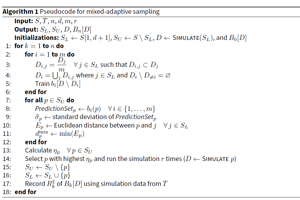
Set \(S\) is further divided into two subsets \(S_{L}\) (labeled points) and \(S_{U}\) (unlabeled points), where a point is labeled if the ABM has been run for that point and unlabeled otherwise. Because all points in \(S\) will be unlabeled initially, they will all start in set \(S_{U}\). Whenever a point \(p\) from \(S_{U}\) is chosen to run the simulation, it is removed from \(S_{U}\) and added to \(S_{L}\). Then, the ABM is initialized according to the input parameter values associated with point \(p\), and it is run for \(r\) replications to capture random variations in the output values. The minimum number of replications needed (\(r\)) can be determined via a variety of different methods, including methods based on variance stability (i.e., tracking when the coefficient of variation or outer variance stabilizes), confidence interval bound variance (i.e., ensuring variability remains within a predefined proportion of a given confidence interval), effect size and power analysis (i.e., controlling Type I and Type II errors by computing the required sample size for detecting a significant difference), and multivariate stability (i.e., accounting for multiple outcomes and parameter sensitivities in complex models) (Lee et al., 2015).
Each design point in set \(S_{L}\) along with the corresponding output data is stored in set \(D\), which will be used to train a ML metamodel represented by \(B_{n}\lbrack D\rbrack\). Specifically, metamodel \(B\) will be trained on the data in set \(D\) for \(n\) iterations of the mixed adaptive algorithm as shown in Algorithm 1. If a new point is added to the set \(S_{L}\), the simulation will be run for the new point, set \(D\) will be updated accordingly, and the metamodel will be retrained. Before implementing the mixed adaptive algorithm, the ABM is also run using the points in test data set \(T\) for \(r\) replications each, and the resulting output data is stored in set \(T\) to evaluate the metamodel (\(B_{n}\lbrack D\rbrack\)) accuracy.
The minimum number of design points required to build an initial metamodel \(B_{0}\lbrack D\rbrack\) must be greater than or equal to the number of input parameters (\(d\)) plus one, so that the model has enough data points to establish meaningful relationships between inputs and outputs. Therefore, to initialize the mixed adaptive sampling algorithm, the ABM is first run on the design points in \(S_{U}\) having an index of 1 to (\(d + 1\)), and \(S_{U}\), \(S_{L},\) and \(D\) are updated accordingly. After this initialization is completed, the algorithm can begin guiding the sequential acquisition of simulation data.
In each iteration of the mixed adaptive sampling algorithm, to select a point from \(S_{U}\) to run the ABM, the point’s quality is evaluated by a process that balances exploitation of the simulation data and exploration of the parameter space. To exploit the data in set \(D\), it is divided into \(m\) mutually exclusive subsets, where \(D_{i}\) represents the \(i^{th}\) stratified subset of \(D\) (lines 2-6). A stratified sample ensures that each design point and its corresponding output data is represented equally in the \(m\) subsets. For example, if the ABM is executed for each design point in \(S_{L}\) with 30 repetitions and \(m = 5\ \)subsets, each \(D_{i}\) is created in such a way that it contains the average of the 6 output values of a given design point in \(S_{L}\) to ensure balanced coverage across repetitions. The \(m\) stratified mutually exclusive subsets of \(D\) are used to train \(m\) sub-models represented by \(b_{i}\lbrack D\backslash D_{i}\rbrack\) where \(b_{i}\) is a ML model trained on set \(D\) excluding \(D_{i}\). For each point \(p\) in \(S_{U}\), a set of \(m\) output predictions are made by the sub-models, denoted as prediction set PredictionSetp (lines 8-9). Prediction uncertainty is then estimated as the standard deviation of the values in PredictionSetp, denoted as \({\widehat{\sigma}}_{p}\) , where higher values imply greater disagreement among the sub-models, indicating nonlinearity (complexity) in the input-output relationship at point \(p\). Prediction uncertainty (\({\widehat{\sigma}}_{p}\)) can be leveraged to identify highly complex regions in the parameter space, which can then be targeted (exploited) for additional simulation runs, ultimately enhancing the metamodel’s prediction accuracy.
However, relying on prediction uncertainty alone to select new points from \(S_{U}\) could lead to oversampling in nonlinear regions of the parameter space. By repeatedly sampling in well-explored nonlinear regions, the algorithm could leave other complex regions underexplored, failing to discover potentially critical relationships and wasting computational resources. To prevent this and encourage exploration of the parameter space, Euclidian distances between each point \(p\) in \(S_{U}\) and the labeled points in \(S_{L}\) are calculated and stored in a set \(E_{p}\). The smallest value in \(E_{p}\) is denoted by \(d_{p}^{\text{min}}\) (lines 10-11), which quantifies the proximity of unlabeled point \(p\) to the labeled points (\(S_{L}\)). Choosing points with the highest values of \(d_{p}^{\text{min}}\) (i.e., those farthest from \(S_{L}\)) and running the ABM using these points to retrain the metamodel enable exploration of regions farther from \(S_{L}\).
To balance the benefits of exploitation and exploration, the quality of point \(p\) is evaluated as \(\eta_{p}\) (line 13) according to Equation (1), where \({\widehat{\sigma}}_{p}\)and \(d_{p}^{\text{min}}\) are normalized with respect to their maximum values among the points in \(S_{U}\). To control the extent of exploration and exploitation by the algorithm, weights \(w_{e}\) (Exploration ratio) and \(w_{x}\) (Exploitation ratio) which add up to 1 are used as shown below.
| \[\begin{equation} \eta_p = w_e\frac{d_p^{\min}}{\max(d_p^{\min})} + w_x\frac{\widehat{\sigma}_p}{\max(\widehat{\sigma}_p)}, \qquad \forall p \in S_U \end{equation}\] | \[(1)\] |
In each iteration of the mixed adaptive sampling algorithm, the point with the highest value of \(\eta_{p}\) is chosen to run the simulation (line 14). The newly acquired data is updated in set \(D\), and point \(p\) is removed from \(S_{U}\) and added to \(S_{L}\) (line 15-16). The model is retrained on updated set \(D\), and this process continues until simulation data on \(n\) new points is acquired, where \(n\) is chosen based on the computational budget.
This formulation mitigates the risk of sampling process being misguided by random noise. Because the uncertainty metric is calculated using ensemble subsets trained on averaged data partitions, random variation from individual simulation runs is filtered out before models are evaluated. Therefore, the disagreement among the sub-models reflects true model ignorance rather than unfair or noisy data partitions. Additionally, the algorithm balances this uncertainty against the spatial nearest-neighbor distance constraint. This distance factor prevents the algorithm from being stuck in localized, noisy areas. Together, these two components ensure that the sampling process is robust and reliably selects points based on a clean mix of data scarcity and spatial gaps.
Case Study 1: Segregation ABM
The Segregation ABM represents two groups of agents residing in a spatial grid (representing a city), in which the agents may choose to relocate in each time-step based on their neighborhood composition preferences, as described by Schelling (1971). The Segregation model has two input parameters: population density (modeled as percentage) and percent similar wanted. The population density parameter determines the percentage of grid cells occupied by agents, and the percent similar wanted parameter specifies the proportion of neighboring agents that an agent expects to be of its own type.
Implementation of sampling algorithms
A random forest machine learning model with 100 decision trees and default values for other hyper-parameters (i.e., maximum depth = none, minimum sample leaf = 1, maximum features = 1.0) was chosen to develop metamodels of the Segregation ABM. A random forest works by building a large collection of independent decision trees using random subsets of data and input features. Each individual tree in the “forest” generates its own prediction based on the specific information it was given. The algorithm then combines these results by averaging them to make a final prediction for a given input parameter combination.
To generate the ABM input parameter combinations, a Sobol’ sequence with 2 input parameters and 6000 design points was generated. The points indexed from 1 to 1000 were assigned to set \(S\), while the remaining points were assigned to set \(T\). Because the Segregation model is a relatively small model and produces outputs with low variability between replications, 30 replications were deemed sufficient, and the mean response was used as the target to train the random forest metamodels.
Pure sequential sampling (SSA), utilizing pure exploitation, was implemented for two different configurations: adding one point per iteration or five points. Mixed adaptive sampling (MASA) was executed with six different ratios of exploration and exploitation weightages while creating five subsets of data (\(m = 5\)) to build the prediction sets. Each experimental scenario was repeated three times using random seeds 30, 120, and 210. Each algorithm ended with the same number of labeled points by the final iteration; for example, an algorithm adding five points per iteration would only require 14 iterations to add 70 labeled points, whereas an algorithm adding one point per iteration would require 70 iterations.
Figure 1 shows the final \(R^{2}\) of all scenarios. It can be observed that SSA always tends to outperform MASA. Furthermore, when the MASA explore/exploit weights are equally balanced at 0.5, there is smaller variation in the metamodel \(R^{2}\).
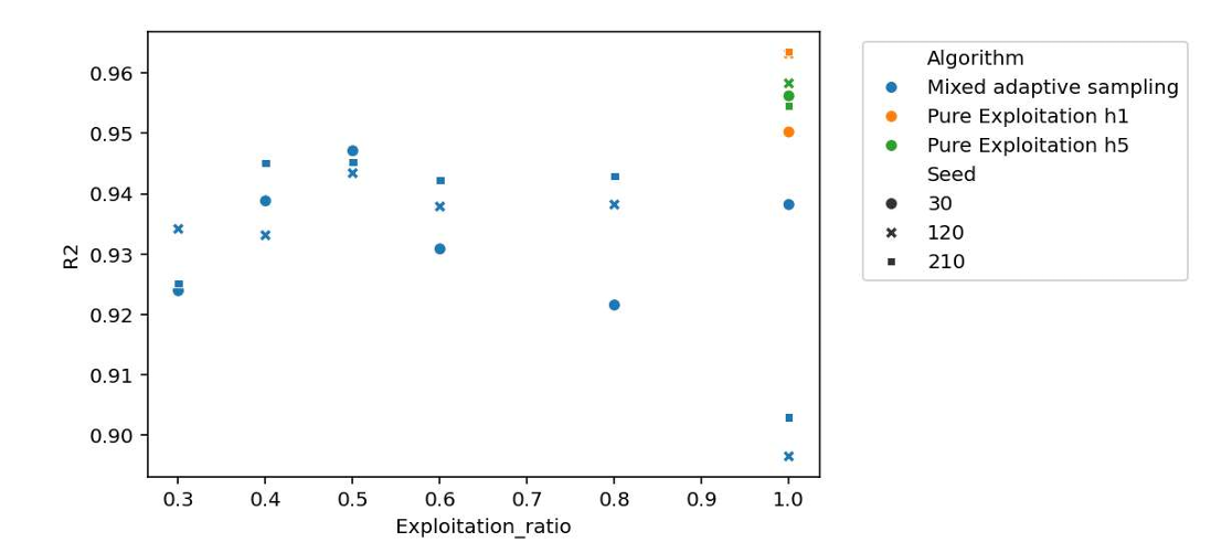
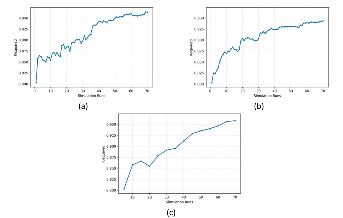
Figure 2 compares the improvement in \(R^{2}\) calculated on test data in each iteration of SSA with one point added per iteration (Figure 2a), MASA with one point added per iteration and the explore/exploit ratio at 0.5/0.5 (Figure 2, panel b), and SSA with five points added per iteration (Figure 2, panel c), all of which used a random seed of 120 (trends for all seeds were similar). The performance of the algorithms when one point is added per iteration stabilizes by 40 iterations, as seen in Figure 2 a and b panels. However, in SSA when five points per iteration are added (Figure 2c), the \(R^{2}\) continues increasing until termination. Furthermore, it can be observed that MASA achieves a higher \(R^{2}\) faster than SSA. As shown in Figure 2, MASA reaches an \(R^{2}\) of approximately 0.9 after about 20 simulations, whereas SSA (Figure 2, panel a and c) remains below this level at the same sampling budget. It is also important to note that adding five points per iteration requires half the run time of SSA and MASA with one point added per iteration. Overall, SSA (\(R^{2} = 96\%)\) slightly outperforms MASA (\(R^{2} = 94.5\%)\).
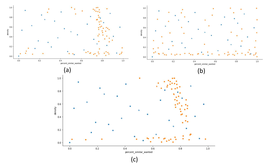
Though MASA with equal weights on exploration and exploitation yields a slightly lower R2 value than SSA, evaluating the points chosen by the algorithms reveals another perspective. Figure 3 plots the initial set of labeled points for which the simulation was run prior to implementing SSA and MASA (shown in blue) and the points chosen by the algorithms (shown in orange), where each point represents a different combination of the ABM input parameters ‘population density’ and ‘percent similar wanted’. Figures 3a and 3c show that SSA results in clustering of points in the nonlinear regions of the parameter space, as previously identified by (Edali & Yücel 2019). However, SSA leaves other regions underexplored. By contrast, MASA with equal explore/exploit weights (Figure 3, panel 3) provides a more even distribution of point selection, indicating that the algorithm maintains global coverage and ensures that the metamodel remains robust across all input combinations. Therefore, MASA learns the entire parameter space while still focusing enough samples on complex nonlinear regions thereby providing a more thorough representation of the ABM’s behavior at the cost of a marginal decrease in peak \(R^{2}\).
Case Study 2: Crowd Logistics ABM
To compare the performance of the sampling algorithms on a larger-scale model, an ABM representing a crowd logistics network with ten input variables was also studied. Crowd logistics is an initiative that provides logistics services (i.e., storage and/or delivery of packages and other items) by using the excess resources and capabilities of a large group of anonymous participants (referred to as the “crowd”), where coordination is enabled by information and technology platforms like websites and mobile applications (Carbone et al. 2017; Mehmann et al. 2015). Crowd logistics has its origin in the term “crowdsourcing” in which tasks (e.g., data collection, content moderation, transportation) are outsourced to individual participants in the crowd (Howe 2006). Participants in a crowd logistics initiative include “senders,” who are seeking delivery services, and “carriers,” who are seeking opportunities to make deliveries for senders in exchange for a fee. A variety of crowd logistics services exist, including Uber Freight, Instacart, Postmates, DropOff, Amazon Flex and DoorDash.
An important phenomenon impacting the growth rate and sustained success (or failure) of crowd logistics platforms is network effects, in which the value of a product, service, or platform depends on the number of buyers, sellers, or users who leverage it (Stobierski 2020). To the senders, the value of the crowd logistics platform increases as carrier participation increases because they are more likely to quickly find a satisfactory carrier, and carriers benefit when there are more senders because there are more work opportunities, which points to indirect network effects (Evans & Schmalensee 2010). When senders and carriers with heterogenous objectives and behaviors interact repeatedly over time via a crowd logistics platform, the resulting complex network dynamics can either lead to platform growth, sustainment, or decline, as participants decide to join or leave the platform.
Thus, it is critical for platform owners to clearly understand the underlying motivations of participants and ensure that their needs are met so that they continue participating and encourage members of their social networks to join, as well. Dynamic participant interactions and feedback loops create complex network effects that make it difficult to predict how participant behaviors on both sides of the platform (i.e., senders and carriers) will affect individuals’ ongoing decisions to continue participating, as well as the likelihood and scale of platform growth and success at the system level. ABM offers the ability to model individual participant attributes, preferences, and dynamic behaviors and then evaluate emergent platform performance metrics over time, making it a particularly useful tool to support the design of successful crowd logistics platforms (Kulkarni & Krejci 2023). (Malan 2022), (Calabrò et al. 2023), and (Cramer & Fikar 2022) have developed ABMs of crowd logistics networks; however, due to the large number of possible parameter settings and computational resource constraints, only a limited number of input parameter combinations were explored.
In previous work, an ABM of a fictitious crowd logistics network was developed (Kulkarni & Krejci 2023) in which senders and carriers are autonomous agents that must repeatedly decide whether or not to participate in the platform. The model’s purpose was to explore how certain parameters (i.e., agent behavior rules and platform characteristics) influence key platform performance metrics (i.e., total number of agents participating and cumulative platform revenue). In each tick (where a tick represents one day), the platform attempts to match senders’ delivery requests with carriers via a matchmaking process based on trip costs, which are calculated using Euclidean distances between a carrier agent’s location and the sender’s desired delivery destination. If there is a suitable match between a carrier and a sender, the carrier makes the delivery on behalf of the sender, who pays for it. The platform earns a portion of this transaction as a commission, which contributes to its revenue. Senders and carriers have heterogeneous attribute values that influence their repeated decisions regarding whether or not to join/leave/continue participating in the platform. More details on the ABM are provided in the Appendix.
Experiments were performed to test the influence of different input parameter values related to platform design and implementation, as well as agent attributes, on carrier/sender participation levels and overall platform revenue over time. One finding from preliminary experimentation with the model was the apparent importance of initial platform participation, suggesting that growth and sustenance of a crowd logistics platform relies heavily on having a critical mass of participants when the platform is launched. However, these conclusions were not robust or definitive, because only a limited set of input parameter configurations were explored; running all combinations of 10 input parameters at different levels for multiple replications proved computationally expensive.
Implementation of sampling algorithms
To address the challenge of experimentation with an ABM having a large parameter space, the sampling algorithms that were tested on the Segregation model (Section 4) were applied to the crowd logistics model. As before, SSA with one and five points added per iteration and MASA with varying explore/exploit weights were used to generate random forest metamodels of the ABM.
To build a reliable ML metamodel which is robust against uncertainty and performs consistently on unseen data, the variability in the ABM output must be represented sufficiently through replication of simulation runs. To determine the minimum number of replications \(r\) that are needed, coefficient of variation (CV) was used. CV normalizes variability relative to the mean, making it applicable to a wide range of distributions without assuming normality. Furthermore, it allows for direct assessment of the stability of output variability by showing how variation in ABM outputs changes as more replications are added. Unlike effect sizes or confidence intervals, which require subjective choices of thresholds to determine number of replications, CV provides a scale-independent measure of variability which naturally converges, indicating when enough replications have been executed, making it particularly useful in ABMs where multiple model outputs on different scales need to be studied simultaneously (Banks et al. 2010). To determine the value of \(r\), a preliminary run of the mixed adaptive algorithm was used to develop a random forest metamodel predicting the ABM output metric “cumulative platform revenue” after 60 simulated days. At \(r = 150\), the coefficient of variation stabilized for both cumulative platform revenue and total platform participation, so 150 replications were deemed sufficient.
Once the number of replications was established, the next step was to execute the sampling algorithms to create the metamodels that would be capable of predicting the two key ABM outputs. Random Forest was used to develop metamodels for ‘Cumulative Platform Revenue’ (\(y_{cpr}\)) using pure sequential sampling with one/five point per iteration (‘Seq1’ and ‘Seq5’) and mixed adaptive sampling with one point per iteration (MAS1) represented by \(R_{Seq1}^{cpr}\lbrack D\rbrack\), \(R_{Seq5}^{cpr}\lbrack D\rbrack\) and \(R_{MAS1}^{cpr}\lbrack D\rbrack\). In parallel, using the simulation data generated by these algorithms, a second metamodel was trained for ‘Total Participation’ (\(y_{tp}\)) represented by \(R_{Seq1}^{tp}\lbrack D\rbrack\), \(R_{Seq5}^{tp}\lbrack D\rbrack\) and \(R_{MAS1}^{tp}\lbrack D\rbrack\). To generate the ABM input parameter combinations, a Sobol’ sequence with 10 input parameters and 2000 design points was generated. The points indexed from 1 to 1500 were assigned to set \(S\), while the remaining points were assigned to set \(T\). The settings used to execute the mixed adaptive sampling and random forest algorithm have been summarized in Table 1.
| Parameter | Description | Value | |
|---|---|---|---|
| Mixed | \(n\) | Number of iterations | 250 |
| \(m\) | Number of sub-models in each iteration | 5 | |
| \(r\) | Number of replications of each design point | 150 | |
| Random Forest | No. of trees | Number of decision trees | 300 |
| Max depth | Max number of levels each tree can grow (if “None,” trees can grow indefinitely) | 8 | |
| Min. sample leaf | Min number of data points required to be in final leaf node | 2 | |
| Max features | Percentage of input features each tree considers at each split | 0.7 | |
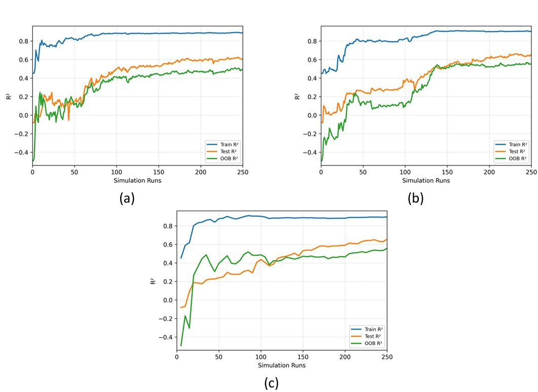
As with the Segregation model, experiments were repeated using three different fixed random seeds. It was also ensured that each algorithm produced the same number of labeled points by the final iteration. Therefore, for SSA and MASA with one point added per iteration, the algorithms were run for 250 iterations, whereas SSA with five points per iteration was run for 50 iterations. Figure 4 compares the improvement in \(R^{2}\) calculated on training, test, and Out of Bag (OOB)) data with each iteration of the algorithms, all of which used a random seed of 120 (trends for all seeds were similar). The OOB \(R^{2}\) is an ensemble-level score where each data point’s prediction is made by aggregating only the trees which excluded that point during training. Figure 4 (panel a and c) shows the results for SSA with 1 and 5 points, respectively, and Figure 4 panel b shows the performance of MASA with weights of 0.45 on exploration and 0.55 on exploitation.
While the high train \(R^{2}\) in comparison to test \(R^{2}\) indicates a degree of overfitting, the model remains effective as the consistently strong and stable test \(R^{2}\) proves that the metamodel has successfully captured the underlying global relationship between inputs and the outputs. As seen in Figure 4 (panel a and c) for SSA, the test \(R^{2}\) is higher than the OOB \(R^{2}\), suggesting the model may be capturing local trends that do not translate as robustly to random internal validation. On the other hand, for MASA, OOB \(R^{2}\) tracks much closer to and occasionally exceeds test \(R^{2}\) as seen in Figure 4 (panel b). This indicates that it explores the design space more thoroughly, thereby creating a model that is globally robust and has learned the underlying structure rather than noise which is just locally accurate to the test set.
Evaluation of algorithms
To be successful, a crowd logistics network must have enough participants (carriers and senders) to consistently make satisfactory matches that earn the platform revenue through transaction fees. To measure the performance of the crowd logistics ABM, the total participation (sum of participating carriers and senders) and the cumulative platform revenue at the end of 60 simulated days (ticks) were tracked. Figure 5 shows the final test \(R^{2}\) values for Cumulative Platform Revenue (\(y_{cpr}\)) using SSA (1 and 5 points) and MASA (exploitation weights set to 0.50, 0.55 and 0.60) with three different seeds (30, 120, and 210). SSA performs similarly to MASA with explore/exploit weights at 0.45 and 0.55, reaching a peak test accuracy value of ~ 65%. It is worth noting that MASA with equal exploitation and exploration weights performs the worst, resulting in 54.9%, 62.2%, and 44.2% for final \(R^{2}\) values.
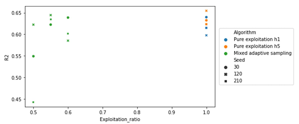
Figure 6 compares the final test accuracy of random forest metamodels for Total Participation (\(y_{tp}\)). As with the random forest metamodels for cumulative platform revenue, metamodels for total participation built using MASA with an exploitation ratio greater than 0.5 give a better test accuracy (approximately 82%). However, in this case SSA slightly underperforms compared to MASA, with an average R2 value of ~ 79%.
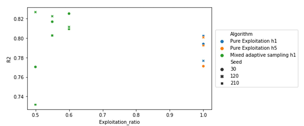
These results indicate that MASA with an exploit weight of 0.55 and an explore weight of 0.45 has the overall best performance and hence was chosen to develop interpretations of the metamodels for both ‘Cumulative Platform Revenue’ (\(y_{cpr}\)) and ‘Total Participation’ (\(y_{tp}\)) in the next section.
Interpretation of results
The relative importance and the effects of changing each of the ten parameters in the crowd logistics ABM were of interest. Accordingly, this section first examines the feature importance of the ten ABM input parameters. Then, for the most important features (input parameters), one-way partial dependence plots are presented, which graphically illustrate the marginal effect of a feature on predicted outcomes while averaging out the effects of all other features. Finally, some key two-way partial dependence plots are presented, which illustrate the joint effect of two features on predicted outcomes.
Feature importance
Feature importance quantifies the degree to which each feature contributes to reducing variance (mean squared error) averaged across all decision trees and is weighted by the number of samples each split affects. This allows the modeler to identify which parameters are the most influential in driving system behavior. Figures 7 and 8 show the feature importance scores for cumulative platform revenue and total participation, respectively. For both performance metrics, “Average decision criteria,” which represents the criteria participants use to decide whether to continue participating with on platform, has highest importance. The second-ranked parameter for total participation is “Average evaluation period,” which represents the number of days agents wait, on average, before making a decision about whether to participate. Second in importance for cumulative platform revenue and fourth for total participation is “Average sender pickup requests,” representing the average number of daily shipment requests created by senders. Indeed, the platform's survival depends on participation, and the decision to participate depends on sufficient opportunities given by shipment requests. However, it should be noted that the top importance score for both metrics is relatively dominant compared to the other features.
“Platform charges,” which represents the percentage of trip cost charged as a fee by the platform, is ranked third in importance for cumulative platform revenue. Third for total participation and fourth for cumulative platform revenue is “Average carrier trip limit,” the average of the maximum number of daily trips a carrier is willing to make, which essentially limits the capacity of the platform to make deliveries. Overall, it is seen that variable importance is primarily focused around 'Decision Criteria’ for total participation, while cumulative platform revenue shows more dependence on the top four parameters. Therefore, the discussion in Section 5.3.2 will consider the top four input features.
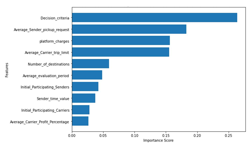
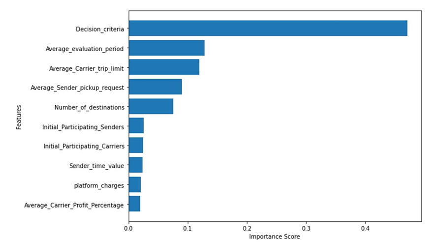
An interesting finding from the feature importance results is that increasing the initial numbers of participating carriers and senders (“Initial carriers” and “Initial senders,” respectively) does not have much effect on the platform’s performance. Indeed, the feature importance results indicate that participants’ characteristics, preferences, and behaviors (e.g., average decision criteria, participation evaluation period, number of sender pickup requests, carrier trip limit) have far greater impact on total participation and total platform revenue than the number of initial participants. Interestingly, these results contradict findings from previous experiments (Kulkarni & Krejci 2022), which suggested that initial participation was an important factor in improving the platform’s odds of success. However, these experiments only tested a specific subset of all possible parameter combinations, and this limited view may have yielded misleading conclusions regarding the relationships between the input parameters and the output metrics. These results emphasize the importance of using an experimental approach that allows for the inclusion of all relevant input parameters when experimenting with an ABM to enable a correct and holistic understanding of the model’s performance and behavior.
Partial dependence plots
The top four features identified by the feature importance analysis for each prediction model were chosen for further analysis using partial dependence plots.
One-Way Partial Dependence Plots
In Figure 9 (panel a), a higher threshold specified for participation decisions leads to lower cumulative platform revenue, where a noticeable drop in revenue occurs when a participant requires more than one match per day to convince them to continue or join. Similarly, Figure 9 (panel b) shows a steep drop in total participation when participants expect more than two matches per day on average. These results suggest that a platform manager should seek to engage participants who expect the platform to provide them with occasional services/jobs, rather than full-time work. However, it seems likely that limiting the participant pool to include only senders and carriers with low expectations would be a barrier to long-term platform growth.
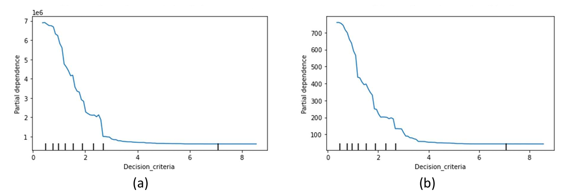
Figure 10 (panel a) shows increasing platform revenue, rising almost linearly with the average number of daily shipment requests created by senders. A significant jump in the revenue can be observed at an average of five sender pickup requests. Figure 10 (panel b) shows similar results for total participation; however, it shows two significant jumps when average daily shipment requests are set to three and five. This indicates that both platform participation and revenue increase dramatically when senders are posting at least five delivery requests every day. This increases the variety of available sender-destination pairs, which improves matching opportunities and enhances carriers' chances of securing matches. One way that a platform manager could increase the volume of daily delivery postings would be to target commercial businesses to participate as senders, since businesses are likely to make frequent and regular shipments to their customers.
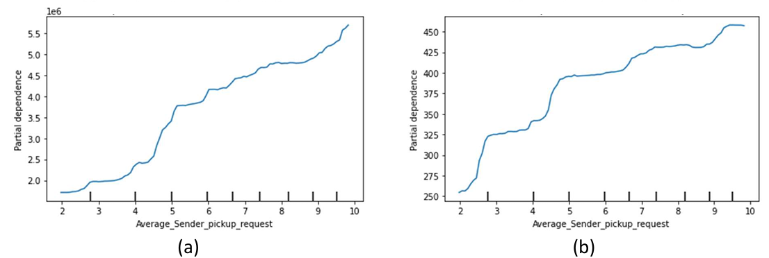
Figure 11 (panel a) shows platform revenue rising strongly beyond an average carrier maximum of four trips per day, before leveling off around five trips per day. On the other hand, Figure 11 (panel b) indicates that participation continues to increase steadily until carriers’ maximum trips exceeds five per day, on average. Together, Figures 10 and 11 suggest that to increase revenue and encourage participation, senders should post at least five requests and carriers should be willing to complete at least four trips per day.
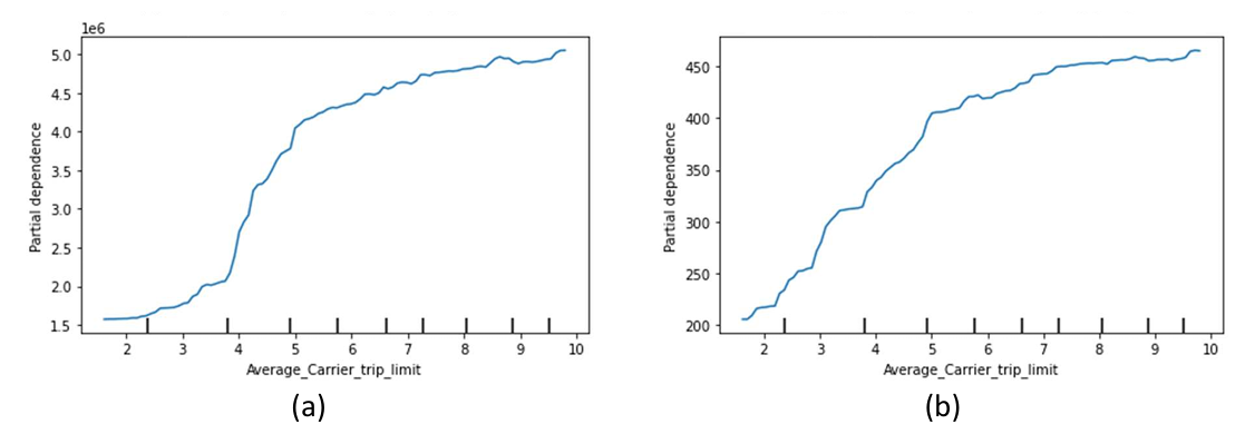
Figure 12 the cumulative platform revenue rises steadily as the number of destinations increases to 30. Since destination expansion has an overall positive impact on revenue (Figure 8), his suggests that the platform should offer more destinations to continuously grow revenue without reaching a visible saturation point.
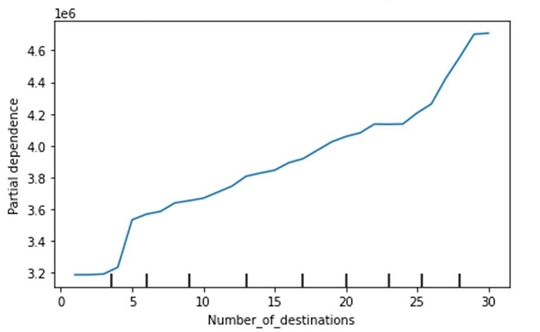
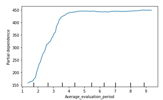
Figure 13 shows that participation increases rapidly after an average evaluation period of two days and plateaus after four days, indicating that when agents make their participation decision based on only one or two days of working for the platform, they are less likely to continue participation.
Two-way Partial Dependence Plots
One-way partial dependence plots reveal the independent effect of a single feature on the model output. However, two-way partial dependence plots are essential for uncovering interactions between features, showing how their combined effect on the model output differs from their individual impact. Thus, two-way partial dependence plots of all possible combinations of the top four important features of the Random Forest model were generated, and a subset of these that indicated interactions and patterns different from the one-way plots were identified.
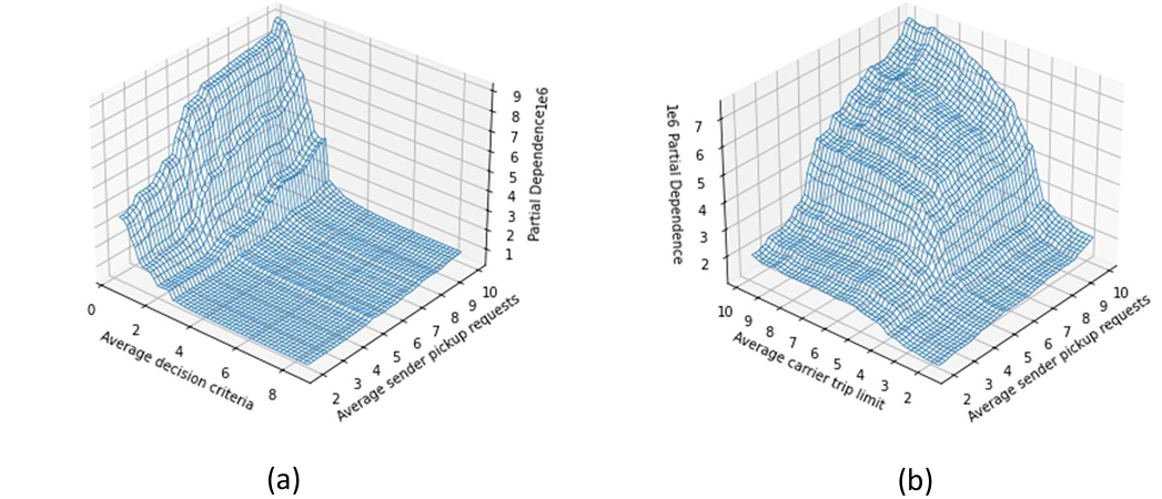
In contrast with the one-way plot in Figure 10 (panel a), which indicates that platform revenue continuously increases with an increasing number of sender pickup requests, Figure 14 (panel a) shows that this is not always the case. Indeed, if the average decision criteria of the participants is greater than 4, this dampens the positive effects of increasing pickup requests and keeps revenue relatively low. However, Figure 14 (panel a) does suggest that having more than 5 pickup requests per sender each day can modestly support cumulative platform revenue, even when the participants’ decision criteria is between 1 and 2.
Furthermore, Figure 14 (panel b) shows that platform revenue only increases with increasing sender pickup requests if the average carrier trip limit is greater than 4, with an abrupt increase when the average carrier trip limit and average sender pickup request values are both greater than 9.
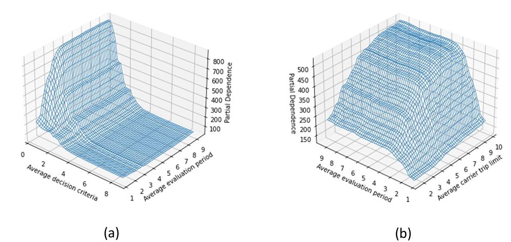
Although Figure 13 indicates that total platform participation increases significantly if participants require more than 3 days to evaluate their participation decision, Figure 15 (panel a) indicates that if the participants’ average decision criteria is greater than 2, average evaluation period does not have much impact on total participation. However, participation drops with a decrease in the average evaluation period if it is less than 4 and the average decision criteria is less than 2.
Figure 11 (panel b) shows that the average carrier trip limit has significant impact on total platform participation only until it reaches 5 trips, which is also observed in the two-way plot shown in Figure 15 (panel b). However, Figure 15 (panel b) provides additional information: when the evaluation period of the participants is below 3 days, the total participation increases only modestly, whereas increasing the average carrier trip limit leads to a much larger rise in participation when the evaluation period exceeds 3 days.
In summary, MASA provided a much deeper understanding of the crowd logistics ABM with just over 750 points (250 points added iteratively and 500 points used to test accuracy of metamodels), which saved significant computational effort.
Conclusion
Large and complex agent-based models have proved to be challenging to analyze, which can limit their usefulness. In an effort to improve computational tractability and interpretation of experimental outputs of such models, this paper evaluates sampling approaches in which a metamodel (Random Forest) is trained iteratively by a mixed adaptive sampling (MASA) and sequential sampling (SSA) algorithms. As these algorithms can be executed under various configurations, experiments with ABMs of segregation model which has two input parameters and the crowd logistics model which has ten input parameters were conducted.
Segregation model results revealed that SSA leads to clustering of points in nonlinear regions due to exploitation. On the other hand, MASA balances exploitation with exploration which ensures good coverage in parameter space while achieving performance comparable to SSA with fewer simulation evaluations. Similar results were observed with the crowd logistics ABM. Feature importance analysis of the revenue and participation metamodels of crowd logistics ABM identified the top four parameters which had the greatest influence on the platform’s performance. Focusing on these top four input parameters, partial dependence plots were then generated, providing insights into the marginal impact of the most important features on the simulation output. Through the techniques used in this study, the development of deeper insights into the impact of agent behavior on the system level performance of an ABM has been made possible in a reasonable number of simulation-runs (750 total runs). Additionally, the experiments conducted in this research could guide ABM modelers in choosing an appropriate sampling method to analyze complex ABMs.
While the metamodeling approach demonstrated in this paper was successful in systematically and efficiently exploring the ABM parameter space, the research does have limitations. Individual conditional expectation plots can be used to highlight instances where the relationship between an input parameter and the predicted simulation output deviates from the general trend, revealing potential interaction effects for further study. Furthermore, the experimentation described in this paper did not establish which parameter settings would yield the highest (i.e., optimal) cumulative platform revenue and total participation. Knowing the optimal parameter settings using techniques such as gradient-boosted optimization, genetic algorithms, or Bayesian optimization would greatly benefit a platform manager by helping them to identify the optimal configuration of the platform.
Appendix
Agent attributes
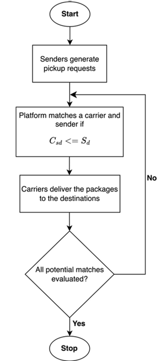
In each tick, senders generate multiple delivery requests, and it is assumed that they are willing to pay a carrier \(S_{d}\) to make a delivery d, where \(S_{d}\)represents a percentage of the amount it would cost the sender to make the delivery themselves. Carriers require a fee of at least \(C_{sd}\) to make a delivery d for sender s, such that a match can only occur between a sender and carrier if \(C_{sd} \leq S_{d}\). However, carriers have a trip limit on the total number of deliveries they are willing to make each day. Based on their level of satisfaction with the number of successful matches the platform finds for them, senders and carriers regularly reevaluate their decision to participate in the platform. This participation decision is based on the agent’s “decision criteria” value, which acts as threshold for the average number of successful matches needed each day for it to be satisfied and continue participating. Each agent also has a set of “friends” within the carrier/sender network that influences its participation decision, based on their satisfaction with the platform.
Initialization and Setup
During setup, 500 senders and 500 carriers are placed at home coordinates, with an experimentally-varied number of randomly-selected carriers and senders that initially participate in the platform. Each agent is assigned a value for the number of “friends” they have of their own kind (i.e., carriers are only friends with other carriers, and senders are only friends with senders), and these friends are randomly assigned to them (Majidi 2023). Destinations to which the senders can request a delivery are created at random coordinates, where the total number of destinations is experimentally varied.
Simulation
At the beginning of each tick, senders generate delivery requests, each of which the platform will attempt to match to a carrier. Figure 16 shows the logic corresponding to a single match, in which a randomly chosen carrier that has not reached its trip limit can match with a randomly chosen sender with outstanding delivery requests only if the carrier’s fee (\(C_{sd}\)) is less than or equal to the sender’s delivery cost (\(S_{d}\)). For carriers, \(C_{sd}\) is calculated by adding the Euclidian distance between the carrier’s current location and the sender’s location to the Euclidian distance between the sender and the destination. This total trip distance is then multiplied with the sum of the carrier’s profit percentage and the platform charge, as shown in Equation 1. Similarly, senders calculate trip cost by multiplying the round-trip distance from their current location to the destination with their time value (i.e., how they value their time), as shown in Equation (2). Equation (3) is used to calculate the revenue generated by the platform during the matchmaking process. To simplify the fictitious ABM, a unit transportation cost of one monetary unit per unit distance was assumed. Consequently, the distance measures appearing in Equations 1–3 are numerically equivalent to transportation costs, ensuring unit consistency throughout the model.
- \(D_{cs}\): Euclidean distance between carrier \(c\) and sender \(s\)
- \(D_{sd}\) : Euclidean distance between sender \(s\) and destination \(d\)
- \(C_{sd}\): Carrier cost for delivering a sender \(s\) delivery to destination \(d\)
- \(S_{d}\): Sender cost to make a delivery to destination \(d\)
- \(R_{csd}\): Platform revenue when carrier \(c\) matches with sender \(s\) for destination \(d\)
- \(C_{p}\): Carrier’s desired profit percentage
- \(P\): Platform charge
- \(S\): Sender’s time value
A carrier agent that matched with a sender will deliver the package and then wait at that location to find a new match. If the carrier finds additional matches, the deliveries will be completed, and the carrier waits at the respective destinations to find more matches. However, if the carrier does not find any matches, the carrier does not move until the matchmaking process has stopped, whereupon it returns to its home location. To ensure efficient matchmaking in each iteration, senders that do not have any more pickup requests remaining and carriers that are unable to find a suitable match or have reached their trip limits are not chosen for matchmaking in the next iteration. This iterative process stops when there are no more potential carriers or senders left to be matched.
Carrier and sender agents track the number of successful matches found for them by the platform in each tick in a “participation history” list. This list is used by the agents to evaluate their participation decision, where the frequency of their participation evaluation is dictated by an “evaluation period” attribute, the value of which varies among agents. During this evaluation, if an agent is not currently participating, it calculates the average number of matches found by its friends and compares it with its own decision criteria value. If the friends’ average number of successful matches is greater than or equal to the agent’s decision criteria value, the agent will decide to begin participating on the platform. On the other hand, if the agent is currently participating on the platform during the evaluation, and if the average number of matches found in its own participation history since the last evaluation is greater than or equal to its decision criteria value, then the agent continues to participate. If this condition is not met, then the agent stops participating on the platform, although it may decide to rejoin in the future if it observes its friends finding successful matches.
To determine how agent attributes and platform characteristics influence the performance of the crowd logistics platform, ten simulation parameters were varied experimentally, as shown in Table 1. Table 1 also shows the scope of the parameter, i.e., the agent or model class affected by that parameter. Each simulation was run for 60 ticks, and at the end of the 60th tick, two responses (i.e., platform performance metric values) were recorded, namely cumulative platform revenue and total current participation on the platform (i.e., number of carriers and number of senders).
| Scope of Parameter | Parameter Name | Description | Parameter Type | Possible Values |
|---|---|---|---|---|
| Model | Initial Carriers | Number of carriers participating on the first day | Discrete | [5,50] |
| Model | Initial Senders | Number of senders participating on the first day | Discrete | [5,50] |
| Model | Number of Destinations | Number of destinations to which senders could request a delivery | Discrete | [1,30] |
| Carriers & Senders | Avg. Evaluation Period | Average no. of days/ticks after which a participants evaluate participation decision | Continuous | [1,10] |
| Carriers | Avg. Trip Limit | Average max no. of trips possible on a given day/tick | Continuous | [1,10] |
| Carriers | Avg. Profit Percentage | Average percentage of delivery cost charged as profit per delivery | Continuous | [3,35] |
| Model | Platform Charges per Delivery | Transaction fee as a percentage of trip distance charged by the platform per match/trip | Continuous | [2,20] |
| Senders | Avg. Delivery Requests | Average daily no. of pickup requests of senders | Continuous | [1,10] |
| Senders | Avg. Time Value | Avg. percentage of delivery cost as a value of time spent in delivering a package | Continuous | [3,35] |
| Carriers & Senders | Avg. Decision Criteria | Average min no. of jobs per day required to alter the participation status during evaluation period | Continuous | [0.25,10] |
References
Ahmed, M., Seraj, R., & Islam, S. M. S. (2020). The k-means algorithm: A comprehensive survey and performance evaluation. Electronics, 9(8). https://doi.org/10.3390/electronics9081295
Alam, M., Deng, X., Philipson, C., Bassaganya-Riera, J., Bisset, K., Carbo, A., Eubank, S., Hontecillas, R., Hoops, S., Mei, Y., Abedi, V., & Marathe, M. (2015). Sensitivity analysis of an ENteric immunity SImulator (ENISI)-based model of immune responses to Helicobacter pylori infection. PLOS ONE, 10(9). https://doi.org/10.1371/journal.pone.0136139
Angione, C., Silverman, E., & Yaneske, E. (2022). Using machine learning as a surrogate model for agent-based simulations. PLOS ONE, 17(2). https://doi.org/10.1371/journal.pone.0263150
Atanassov, E., Ivanovska, S., & Karaivanova, A. (2021). Optimization of the direction numbers of the Sobol sequences. In I. Dimov & S. Fidanova (Eds.), Advances in high performance computing (pp. 145–154). Springer International Publishing. https://doi.org/10.1007/978-3-030-55347-0_13
Azmin, F. M., & Stobart, R. (2015). Benefiting from Sobol sequences experiment design type for model-based calibration (SAE Technical Paper No. 2015-01-1640). SAE International. https://doi.org/10.4271/2015-01-1640
Banks, J., Carson, J. S., Nelson, B. L., & Nicol, D. M. (2010). Discrete_event system simulation. Pearson Education.
Barton, R. R. (2020). Tutorial: Metamodeling for simulation. 2020 Winter Simulation Conference (WSC), 1102–1116. https://doi.org/10.1109/WSC48552.2020.9384059
Bhattacharjee, S., MacPherson, B., Wang, R. F., & Gras, R. (2019). Animal communication of fear and safety related to foraging behavior and fitness: An individual-based modeling approach. Ecological Informatics, 54. https://doi.org/10.1016/j.ecoinf.2019.101011
Bose, R. C., & Bush, K. A. (1952). Orthogonal arrays of strength two and three (No. 4; Vol. 23, pp. 508–524). The Annals of Mathematical Statistics. https://doi.org/10.1214/aoms/1177729331
Breiman, L. (2001). Random Forests. Machine Learning, 45(1), 5–32. https://doi.org/10.1023/A:1010933404324
Breiman, L., Friedman, J., Olshen, R. A., & Stone, C. J. (2017). Classification and regression trees. Chapman; Hall/CRC. https://doi.org/10.1201/9781315139470
Broeke, G. ten, Voorn, G. van, & Ligtenberg, A. (2016). Which sensitivity analysis method should i use for my agent-based model? Journal of Artificial Societies and Social Simulation, 19(1), 5.
Burhenne, S., Jacob, D., & Henze, G. P. (2011). Sampling based on Sobol’ sequences for Monte Carlo techniques applied to building simulations. Building Simulation, 12, 1816–1823. https://doi.org/10.26868/25222708.2011.1590
Calabrò, G., Le Pira, M., Giuffrida, N., Fazio, M., Inturri, G., & Ignaccolo, M. (2023). A spatial agent-based model of e-commerce last-mile logistics towards a delivery-oriented development. Transportation Research Interdisciplinary Perspectives, 21. https://doi.org/10.1016/j.trip.2023.100895
Carbone, V., Rouquet, A., & Roussat, C. (2017). The rise of crowd logistics: A new way to co-create logistics value. Journal of Business Logistics, 38(4), 238–252. https://doi.org/10.1111/jbl.12164
Cervantes, J., Garcia-Lamont, F., Rodríguez-Mazahua, L., & Lopez, A. (2020). A comprehensive survey on support vector machine classification: Applications, challenges and trends. Neurocomputing, 408, 189–215. https://doi.org/10.1016/j.neucom.2019.10.118
Chang, S., Kato, T., Koyanagi, Y., Uemura, K., & Maruhashi, K. (2023). An iterative analysis method using causal discovery algorithms to enhance ABM as a policy tool. 2023 Winter Simulation Conference (WSC), 138–149. https://doi.org/10.1109/WSC60868.2023.10407967
Chen, S. H., Londoño-Larrea, P., McGough, A. S., Bible, A. N., Gunaratne, C., Araujo-Granda, P. A., Morrell-Falvey, J. L., Bhowmik, D., & Fuentes-Cabrera, M. (2021). Application of Machine Learning techniques to an agent-based model of Pantoea. Frontiers in Microbiology, 12. https://doi.org/10.3389/fmicb.2021.726409
Chen, T., & Guestrin, C. (2016). XGBoost: A scalable tree boosting system. Proceedings of the 22nd ACM SIGKDD International Conference on Knowledge Discovery and Data Mining, KDD ’16, 785–794. https://doi.org/10.1145/2939672.2939785
Chen, V. C. P., Tsui, K.-L., Barton, R. R., & Meckesheimer, M. (2006). A review on design, modeling and applications of computer experiments. IIE Transactions, 38(4), 273–291. https://doi.org/10.1080/07408170500232495
Cheng, Y., Li, L., Xiao, T., Li, Z., Suo, J., He, K., & Dai, Q. (2024). CUTS+: High-dimensional causal discovery from irregular time-series. Proceedings of the AAAI Conference on Artificial Intelligence, 38. https://doi.org/10.1609/aaai.v38i10.29034
Cohn, D., Atlas, L., & Ladner, R. (1994). Improving generalization with active learning. Machine Learning, 15(2), 201–221. https://doi.org/10.1007/BF00993277
Cramer, F., & Fikar, C. (2022). Simulating the viability of crowd logistics in short food supply chains. 26th ASIM Symposium Simulationstechnik, 19, 17–20. https://www.asim-gi.org/fileadmin/user_upload_asim/ASIM_Publikationen_OA/AM179/arep.19_OA.pdf
Crombecq, K., De Tommasi, L., Gorissen, D., & Dhaene, T. (2009). A novel sequential design strategy for global surrogate modeling. Proceedings of the 2009 Winter Simulation Conference (WSC), 731–742. https://doi.org/10.1109/WSC.2009.5429687
Crombecq, K., Laermans, E., & Dhaene, T. (2011). Efficient space-filling and non-collapsing sequential design strategies for simulation-based modeling. European Journal of Operational Research, 214(3), 683–696. https://doi.org/10.1016/j.ejor.2011.05.032
Dean, A., & Voss, D. (1999). Fractional factorial experiments. In Design and analysis of experiments (pp. 483–545). Springer. https://doi.org/10.1007/0-387-22634-6_15
Dooley, K. (1996). Complex adaptive systems: A nominal definition. The Chaos Network, 8(1), 2–3.
Eason, J., & Cremaschi, S. (2014). Adaptive sequential sampling for surrogate model generation with artificial neural networks. Computers & Chemical Engineering, 68, 220–232. https://doi.org/10.1016/j.compchemeng.2014.05.021
Edali, M., & Yücel, G. (2019). Exploring the behavior space of agent-based simulation models using random forest metamodels and sequential sampling. Simulation Modelling Practice and Theory, 92, 62–81. https://doi.org/10.1016/j.simpat.2018.12.006
Evans, D. S., & Schmalensee, R. (2010). Failure to launch: Critical mass in platform businesses. SSRN. https://dspace.mit.edu/handle/1721.1/76685
Fang, K.-T., & Wang, Y. (1993). Number-theoretic methods in statistics. CRC Press.
Frasca, M., La Torre, D., Pravettoni, G., & Cutica, I. (2024). Explainable and interpretable artificial intelligence in medicine: A systematic bibliometric review. Discover Artificial Intelligence, 4(1). https://doi.org/10.1007/s44163-024-00114-7
Friedman, J. H. (2001). Greedy function approximation: A gradient boosting machine. The Annals of Statistics, 29(5), 1189–1232.
Friedman, L. W., & Pressman, I. (1988). The metamodel in simulation analysis: Can it be trusted? Journal of the operational research society, 39(10), 939–948. https://doi.org/10.1057/jors.1988.160
Garg, A., Yuen, S., Seekhao, N., Yu, G., Karwowski, J. A. C., Powell, M., Sakata, J. T., Mongeau, L., JaJa, J., & Li-Jessen, N. Y. K. (2019). Towards a physiological scale of vocal fold agent-based models of surgical injury and repair: Sensitivity analysis, calibration and verification. Applied Sciences, 9(15). https://doi.org/10.3390/app9152974
Holland, J. H. (1992). Complex adaptive systems. Daedalus, 121(1), 17–30.
Howe, J. (2006). The rise of crowdsourcing. Wired. https://www.wired.com/2006/06/crowds/
Huber, M. (2024). An introduction to causal discovery. Swiss Journal of Economics and Statistics, 160(1). https://doi.org/10.1186/s41937-024-00131-4
Hussain, Mohd. S., & Ali, M. (2019). A multi-agent based dynamic scheduling of flexible manufacturing systems. Global Journal of Flexible Systems Management, 20(3), 267–290. https://doi.org/10.1007/s40171-019-00214-9
James, L. P., Salomon, J. A., Buckee, C. O., & Menzies, N. A. (2021). The use and misuse of mathematical modeling for infectious disease policymaking: Lessons for the COVID-19 pandemic. Medical Decision Making, 41(4), 379–385. https://doi.org/10.1177/0272989X21990391
Janssen, S., Sharpanskykh, A., Curran, R., & Langendoen, K. (2019). Using causal discovery to analyze emergence in agent-based models. Simulation Modelling Practice and Theory, 96. https://doi.org/10.1016/j.simpat.2019.101940
Kasaie, P., & Kelton, W. D. (2015). Guidelines for design and analysis in agent-based simulation studies. 2015 Winter Simulation Conference (WSC), 183–193. https://doi.org/10.1109/WSC.2015.7408163
Kulkarni, P., & Krejci, C. (2022). Evaluating a Crowd Logistics Network Using Agent-Based Modeling. Conference of the Computational Social Science Society of the Americas (pp. 21-34). Cham: Springer International Publishing. https://doi.org/10.1007/978-3-031-37553-8_2
Kulkarni, P., & Krejci, C. C. (2023). Matchmaking in Crowd-Shipping Platforms: The Effects of Mediator Control. Proceedings Winter Simulation Conference. IEEE. https://doi.org/10.1109/WSC60868.2023.10407822
Larie, D., An, G., & Cockrell, R. C. (2021). The use of artificial neural networks to forecast the behavior of agent-based models of pathophysiology: An example utilizing an agent-based model of sepsis. Frontiers in Physiology, 12. https://doi.org/10.3389/fphys.2021.716434
Lee, J.-S., Filatova, T., Ligmann-Zielinska, A., Hassani-Mahmooei, B., Stonedahl, F., Lorscheid, I., Voinov, A., Polhill, J. G., Sun, Z., & Parker, D. C. (2015). The complexities of agent-based modeling output analysis. Journal of Artificial Societies and Social Simulation, 18(4). https://doi.org/10.18564/jasss.2897
Li, L., Wang, J., Zhong, X., Lin, J., Wu, N., Zhang, Z., Meng, C., Wang, X., Shah, N., Brandon, N., Xie, S., & Zhao, Y. (2022). Combined multi-objective optimization and agent-based modeling for a 100% renewable island energy system considering power-to-gas technology and extreme weather conditions. Applied Energy, 308. https://doi.org/10.1016/j.apenergy.2021.118376
Liu, H., Ong, Y.-S., & Cai, J. (2018). A survey of adaptive sampling for global metamodeling in support of simulation-based complex engineering design. Structural and Multidisciplinary Optimization, 57(1), 393–416. https://doi.org/10.1007/s00158-017-1739-8
Liu, R. (2022). Studies of COVID-19 outbreak control using agent-based modeling [Master’s thesis, The University of Iowa]. https://www.proquest.com/docview/2694335044/abstract/C00F72BD49E446EDPQ/1
Majidi, M. (2023). Number of close friends had by U.S. Adults 2021. Statista. https://www.statista.com/statistics/1358672/number-of-close-friends-us-adults/
Malan, P. C. (2022). An agent-based approach to customer crowd-shipping [Master’s thesis]. http://hdl.handle.net/10019.1/124680
Marchi, S. de, & Page, S. E. (2014). Agent-based models. Annual Review of Political Science, 17(1), 1–20. https://doi.org/10.1146/annurev-polisci-080812-191558
Mehmann, J., Frehe, V., & Teuteberg, F. (2015). Crowd logistics − a literature review and maturity model. In Innovations and strategies for logistics and supply chains: Technologies, business models and risk management. Proceedings of the hamburg international conference of logistics (HICL), vol. 20 (pp. 117–145). Berlin: epubli GmbH. https://www.econstor.eu/handle/10419/209253
Musolf, A. M., Holzinger, E. R., Malley, J. D., & Bailey-Wilson, J. E. (2022). What makes a good prediction? Feature importance and beginning to open the black box of machine learning in genetics. Human Genetics, 141(9), 1515–1528. https://doi.org/10.1007/s00439-021-02402-z
Nagel, K., & Schreckenberg, M. (1992). A cellular automaton model for freeway traffic. Journal de Physique I, 2(12), 2221–2229. https://doi.org/10.1051/jp1:1992277
Ozik, J., Collier, N. T., Wozniak, J. M., Macal, C. M., & An, G. (2018). Extreme-scale dynamic exploration of a distributed agent-based model with the EMEWS framework. IEEE Transactions on Computational Social Systems, 5(3), 884–895. https://doi.org/10.1109/TCSS.2018.2859189
Papacharalampous, G., Tyralis, H., Doulamis, A., & Doulamis, N. (2023). Comparison of tree-based ensemble algorithms for merging satellite and earth-observed precipitation data at the daily time scale. Hydrology, 10(2). https://doi.org/10.3390/hydrology10020050
Pereda, M., Santos, J. I., & Galán, J. M. (2017). A brief introduction to the use of Machine Learning techniques in the analysis of agent-based models. In C. Hernández (Ed.), Advances in management engineering (pp. 179–186). Springer International Publishing. https://doi.org/10.1007/978-3-319-55889-9_11
Platas-López, A., Guerra-Hernández, A., Quiroz-Castellanos, M., & Cruz-Ramirez, N. (2023). A survey on agent-based modelling assisted by machine learning. Expert Systems, n/a(n/a). https://doi.org/10.1111/exsy.13325
Quinlan, J. R. (1986). Induction of decision trees. Machine Learning, 1(1), 81–106. https://doi.org/10.1007/BF00116251
R. Vahdati, A., Weissmann, J. D., Timmermann, A., Ponce de León, M. S., & Zollikofer, C. P. E. (2019). Drivers of late pleistocene human survival and dispersal: An agent-based modeling and machine learning approach. Quaternary Science Reviews, 221. https://doi.org/10.1016/j.quascirev.2019.105867
Rasmussen, C. E. (2004). Gaussian processes in Machine Learning. In U. von L. O. Bousquet & G. Rätsch (Eds.), Advanced lectures on machine learning: ML summer schools 2003, canberra, australia, february 2–14, 2003, tübingen, germany, august 4–16, 2003, revised lectures (pp. 63–71). Springer. https://doi.org/10.1007/978-3-540-28650-9_4
Saltelli, A., Aleksankina, K., Becker, W., Fennell, P., Ferretti, F., Holst, N., Li, S., & Wu, Q. (2019). Why so many published sensitivity analyses are false: A systematic review of sensitivity analysis practices. Environmental Modelling & Software, 114, 29–39. https://doi.org/10.1016/j.envsoft.2019.01.012
Saltelli, A., Ratto, M., Andres, T., Campolongo, F., Cariboni, J., Gatelli, D., Saisana, M., & Tarantola, S. (2008). Global sensitivity analysis: The primer. John Wiley & Sons.
Schelling, T. C. (1971). Dynamic models of segregation†. The Journal of Mathematical Sociology, 1(2), 143–186. https://doi.org/10.1080/0022250X.1971.9989794
Shao, Z., Ahmad, M. N., & Javed, A. (2024). Comparison of Random Forest and XGBoost classifiers using integrated optical and SAR features for mapping urban impervious surface. Remote Sensing, 16(4). https://doi.org/10.3390/rs16040665
Sloane, N. J. A. (2012). Orthogonal arrays. http://neilsloane.com/oadir/
Sobol, I. M. (1967). The distribution of points in a cube and the approximate evaluation of integrals. U. S. S. R. Computational Mathematics and Mathematical Physics, 7, 86–112.
Sobol′, I. M. (2001). Global sensitivity indices for nonlinear mathematical models and their Monte Carlo estimates. Mathematics and Computers in Simulation, The Second IMACS Seminar on Monte Carlo Methods, 55(1), 271–280. https://doi.org/10.1016/S0378-4754(00)00270-6
Srbljinović, A., & Škunca, O. (2003). AN INTRODUCTION TO AGENT BASED MODELLING AND SIMULATION OF SOCIAL PROCESSES. Interdisciplinary Description of Complex Systems, 1, 1–2.
Stobierski, T. (2020). What are network effects? | HBS online. Business insights blog. https://online.hbs.edu/blog/post/what-are-network-effects
Venugopalan, J., Deshkar, G., Kshirsagar, J., Singh, D., Jose, J., & Hayatnagarkar, H. (2023). Agent-based model output analysis – a comprehensive statistical framework. 2023 Annual Modeling and Simulation Conference (ANNSIM), 25–36. https://ieeexplore.ieee.org/abstract/document/10155359