 Abstract
- The proliferation of agent-based models (ABMs) in recent
decades has motivated model practitioners to improve the transparency,
replicability, and trust in results derived from ABMs. The complexity
of ABMs has risen in stride with advances in computing power and
resources, resulting in larger models with complex interactions and
learning and whose outputs are often high-dimensional and require
sophisticated analytical approaches. Similarly, the increasing use of
data and dynamics in ABMs has further enhanced the complexity of their
outputs. In this article, we offer an overview of the state-of-the-art
approaches in analysing and reporting ABM outputs highlighting
challenges and outstanding issues. In particular, we examine issues
surrounding variance stability (in connection with determination of
appropriate number of runs and hypothesis testing), sensitivity
analysis, spatio-temporal analysis, visualization, and effective
communication of all these to non-technical audiences, such as various
stakeholders.
- Keywords:
- Agent-Based Modelling, Methodologies, Statistical Test, Sensitivity Analysis, Spatio-Temporal Heterogeneity, Visualization
 Introduction
- 1.1
- Agent-based models (ABMs) have been gaining popularity
across disciplines and have become increasingly sophisticated. The last
two decades have seen excellent examples of ABM applications in a broad
spectrum of disciplines including ecology (Grimm
& Railsback 2005; Thiele
& Grimm 2010), economics (Kirman
1992; Tesfatsion
& Judd 2006), health care (Effken
et al. 2012), sociology (Macy
& Willer 2002; Squazzoni
2012), geography (Brown
& Robinson 2006), anthropology (Axelrod & Hammond 2003),
archaeology (Axtell et al. 2002),
bio-terrorism (Carley et al. 2006),
business (North & Macal 2007),
education (Abrahamson et al. 2007),
medical research (An & Wilensky
2009), military tactics (Ilachinski
2000), neuroscience (Wang et
al. 2008), political science (Epstein
2002), urban development and land use (Brown
et al. 2005), and zoology (Bryson
et al. 2007). This methodology now also penetrates
organizational studies (Carley
& Lee 1998; Lee
& Carley 2004; Chang
& Harrington 2006), governance (Ghorbani et al. 2013), and is
becoming actively employed in psychology and other behavioural studies,
exploiting data from laboratory experiments and surveys (Duffy 2006; Contini et al. 2007; Klingert & Meyer 2012).
- 1.2
- ABMs produce a rich set of multidimensional data on macro
phenomena, comprising a myriad of details on micro-level agent choices
and their dynamic interactions at various temporal and spatial
resolutions. Despite significant progress made in empirically grounding
ABM mechanisms and agent attributes (Robinson
et al. 2007; Windrum et
al. 2007; Smajgl et al.
2011), ABMs continue to harbour a considerable amount of
subjectivity and hence degrees of freedom in the structure and
intensity of agents' interactions, agents' learning and adaptation, and
any potential thresholds affecting switching in strategies. The
increasing complexity of ABMs has been further stimulated by improvements
in computing technology and wider availability of advanced computing
resources. These qualities demand a comprehensive (or at least
sufficient) exploration of the model's behaviour.
- 1.3
- To complicate matters further, an ABM is typically a stochastic
process and thus requires Monte Carlo sampling, in which
each experiment (or parameter setting) is multiply performed using
distinct pseudo-random sequences (i.e., different random seeds) in
order to achieve the statistical robustness necessary for testing
hypotheses and distinguishing multiple scenarios under varying
experimental or parameter settings. By "random seed", we mean the seed
for the random number generator. Thus, an ABM delivers a high volume of
output data rendering the identification of salient and relevant
results (such as trends) and the assessment of model sensitivities to
varying experimental conditions a challenging problem.
- 1.4
- All these complications apply not only to the analysis of
ABM output data but also to the model's design and implementation. The
massive diversity in outputs, often exhibiting temporal and spatial
dimensions, necessitates judicious model design, planning, and
application. Poor or unstructured design may lead to unnecessarily
larger outputs to reach the same (or even less) precise conclusions
that one may infer from outputs of well-designed models and
experimentation. The standards employed in the ABM field, such as ODD
(Overview, Design concepts, and Details) (Grimm
et al. 2006, 2010;
Müller et al. 2013)
and DOE (design of experiments) (Fisher
1971), have significantly improved transparency,
replicability, and trust in ABM results. However, the field continues
to lack specific guidance on effective presentation and analysis of ABM
output data, perhaps due to this issue's having less priority in ABM
social science research or due to technical barriers. Furthermore,
converging on universal standards remains elusive partly due to the
broad spectrum of research fields employing ABMs. Domain-relevant
metrics, analytical techniques, and communication styles are largely
driven by each discipline's target audience.
- 1.5
- Yet, there are common methodological challenges facing ABM
modellers in their path toward understanding, refining, and distilling
the most relevant and interesting results from a nearly-endless sea of
output data. While a modeller invests a significant amount of time and
effort in the development of an ABM itself, a comprehensive or
compelling analysis of the ABM output data is not always considered as
deserving the same resource-intensive attention. Proper output analysis
and presentation are vital for developing a domain-specific message
containing innovative contributions.
- 1.6
- This paper aims to provide an overview of the
state-of-the-art in how agent-based modellers contend with their model
outputs, their statistical analysis, and visualization techniques.[1] We discuss challenges
and offer examples for addressing them. The first topic deals with
several issues surrounding the study of variance in the model outputs
(i.e., stability) and its impact on both model design (e.g., simulation
runs or "samples") and analysis (e.g., hypothesis testing). The next
one addresses the state of sensitivity analysis and the complexities
inherent in the exploration of the space that encapsulates both the
parameters and the outcomes. The third topic focuses on the analysis
and presentation of spatial (including geospatial) and temporal results
from ABMs.
- 1.7
- We also survey the role of effective visualization as a medium for both analysis and exposition of model dynamics. Comments on visualization appear within each main topic as visualization strategies tend to be strongly defined and constrained by the topic matter. Finally, we outline outstanding issues and potential solutions which are deemed as future work for ourselves and other researchers.
 Determining
Minimum Simulation Runs and Issues of Hypothesis Testing
- 2.1
- ABM researchers strive to expose important and relevant
elements in their models' outputs and consequently the underlying
complex dynamics in both quantitative and qualitative ways. Compelling
statements about an ABM's behaviours may be drawn from descriptive
statistics of distinct outcomes (e.g., mean and standard deviation) or
statistical tests in which outcomes are compared (e.g., t-test),
predicted (in the statistical sense, e.g., multiple regression), or
classified (e.g., clustering or principal component analysis). Given the
stochastic nature of most ABMs, these analytical exercises require an
outcome pool drawn from a sufficient number of samples (i.e.,
simulation runs).
- 2.2
- The quantity of ABM output samples has several
ramifications to experimental design and the quality of the analysis.
For those large and complex ABMs whose longer run times prohibit the production
of large samples, the relevant question is the minimum number of
required runs. Conversely, expedient ABMs offer the temptation of
producing far greater sample counts thereby increasing the sensitivity
of statistical tests possibly to the point of absurdity. That is, one
might produce so many samples such that traditional tests expose
extremely small and contextually inconsequential differences. We focus
our discussion on the methods for the determining the number of minimum
runs. Implications of having too many samples are discussed in Appendix
B.
Minimum Sample Size (Number of Runs)
- 2.3
- The determination of the minimum sample size partly relies
on the analytical objective. One common objective is a statistical
description of the outcomes typically in the form of means and standard
deviations (or alternatively, variances). Since the shape of a
model's output distributions are usually a priori unknown,
the point or sample size at which outcome mean and variance reaches
relative quiescence or stability is crucial to accurate reporting of
the descriptive statistics. Otherwise, the statistics would harbour too
much uncertainty to be reliable. Unfortunately, all of the different
criteria for determining this point of stability suffers from some
degree of subjectivity, and thus it falls on the analyst to wisely make
the selection. Furthermore, these approaches appear to remain either
underused or unknown to many ABM researchers (Hamill
2010). In fact, a survey of some of ABM literature reveals
sample sizes to be too low, conveniently selected (sample sizes of 100
or less are common), or exorbitantly high (Angus
& Hassani-Mahmooei 2015).
Variance Stability
- 2.4
- Assessing variance stability requires a metric to measure
the uncertainty surrounding the variance (or the variance of variance
if you will). Law and Kelton (2007)
and Lorscheid et al. (2012)
offer such metrics both of which rely on some functional ratio between
the variance and the sample mean. Law & Kelton's approach seeks
a sample size in which the variability remains within some predefined
proportion of the confidence interval around the mean (confidence
interval bound variance), thus it is bound to the
assumptions of normality, namely that the mean has a Gaussian
distribution. Hence, the researcher must select this proportion from
outputs of a trial set of runs. Lorscheid et al.'s method eschews those
assumptions by employing the coefficient of
variation and a fixed epsilon
(\(E\)) limit of that metric. While these are dimensionless metrics,
their use is problematic for simulation studies in which multivariate
outcomes from parameter effects are analyzed.
- 2.5
- The coefficient of variation is simply the ratio of the
standard deviation of a sample (\(\sigma\)) to its mean (\(\mu\)):
$$ c_V^{\phantom{x}}=\frac{\sigma}{\mu} $$ - 2.6
- This scaling offers a similar interpretation as the
confidence interval (C.I.): \(c_V^{\phantom{x}} \rightarrow 0\) is
equivalent to \(t(0 \notin \mathrm{C.I.}) \rightarrow \infty\) and the
\(p\)-value approaches 0. That is, when the standard deviation shrinks
relative to the mean, the probability of the confidence interval
spanning across the value of 0 drops precipitously. The coefficient of
variation (\(c_V^{\phantom{x}}\)) will exhibit substantial variance for
small sample sizes just like the standard error of the mean. For
example, the \(c_V^{\phantom{x}}\) of a single ABM outcome obtained
from a set of five runs will vary more with the same metrics taken from
other sets of five runs than if each set contained far more runs, say
100. Lorscheid et al. compare the \(c_V^{\phantom{x}}\)'s of
differently sized sets of runs (e.g., the \(c_V^{\phantom{x}}\) from 10
runs, then 100, 500, and so forth). The sample size at which the
difference between consecutive \(c_V^{\phantom{x}}\)'s falls below a
criterion, \(E\), and remains so is considered a minimum sample size or
minimum number of ABM runs. For example, if an outcome drawn from runs
of different sample sizes, \(n \in\{10, 500, 1000, 5000, 10000\}\),
yields the \(c_V^{\phantom{x}}\)'s (rounded to 1/100) \(\{0.42, 0.28,
0.21, 0.21, 0.21\}\) and we select \(E = 0.01\), we would consider the
third sample size (\(n = 1000\)) as the point of stability. These
\(c_V^{\phantom{x}}\) stability points are obtained for all ABM
outcomes of interest (in a multivariate setting), and thus the minimum
number of runs for the ABM is the maximum of these points:
$$ n_{\min} = {\mathop{\rm argmax}\limits}_{n} | c_V^{x,n} - c_V^{x,m}| < E,~\forall x~\mathrm{and}~\forall m>n $$ where \(n_{\min}\) is the estimated minimum sample size; \(x\) is a distinct outcome of interest; and \(m\) is some sample size \(> n\) for which the \(c_V^{\phantom{x}}\) (of each outcome) is measured.
- 2.7
- However, the fixed \(E\) favors those \(\mu\) sufficiently
larger than 0 and also larger than its corresponding \(\sigma\) and
penalizes \(n_{\min}\) for outcomes with \(\mu\) closer to 0. That is,
the more likely an outcome's confidence interval encompasses 0, the
erroneously larger the estimation of \(n_{\min}\) will be. Conversely,
the fixed \(E\) renders the procedure too effective and results in an
underestimation of \(n_{\min}\) for those C.I.'s that reside far from 0,
relative to \(\sigma\). Therefore, we urge some caution in using
\(c_V^{\phantom{x}}\) to determine the minimum sample size and applying
it only to ABMs for which the outcomes of interest are prejudiced
against attaining a value of 0. As such, Lorscheid et al.'s approach
determines a minimum sample size not just based on variance stability
but also the likelihood an outcome's confidence interval contains 0.
- 2.8
- Alternatively, one might consider just variance stability
without any consideration of the mean value. Following Lorscheid et
al.'s strategy of assessing stability from metrics on an outcome for a
sequence of sample sizes, we track the windowed
variance of simple outcomes from several canonical
statistical distributions as well as an ABM model. The distributions we
employ here for demonstration purposes are the normal (or Gaussian),
uniform, exponential, Poisson, \(\chi^2\), and t
distributions.[2]
While ABM outputs do not always conform to one of these parametric
distributions, the ones we examine here are distinct enough to provide
us with a sense of variance stability for a spectrum of distributions.
These distributions will serve as proxies for ABMs' outcomes and, for
our purposes, have been parameterized so that their theoretical
variance \(\sigma^2\approx 1\). We also include an outcome from a
simple ABM model of Birth Rates (Wilensky
1997). This ABM entails two dynamically changing
populations (labelled "red" and "blue"). Here, our outcome is the size
of the "red" population. For further details, see Figure 17 in
Appendix C.
- 2.9
- In Figure 1a, we
offer variances for varying sized samples of Gaussian variates (i.e.,
scalars drawn from the Gaussian distribution parameterized to have a
variance of 1). At low sample sizes, there is considerable variance
surrounding the sample variance itself as evidenced by the "noisiness"
of the variance from one sample size to the next. After a certain point
(roughly \(n = 400\)), this outer variance
appears to stabilize and continues to further converge to 0 albeit
slowly.
- 2.10
- The outer variance at each sample size can then be measured
using the variance of proximal sample sizes. For example, the outer
variance for \(n = 10\) is calculated from variance of the sample
variances of \(n\in\{10,\ldots, 10+(W-1)g\}\), where \(W\) is some
predetermined size of the window and \(g\) is our sample size
increment; we select \(g=W=10\), and we so consider
\(n\in\{10,20,\ldots,100\}\) for the variance surrounding \(n=10\).
Notationally, this outer variance may be expressed as \(\sigma^2\)
(\(s^2\)) but given its estimation using windows, we assign it
\(\omega_n^2\), where \(n\) is the sample size. In Figure 1, we chart the \(\omega_n^2\)
relative to its maximum value (\(\frac{\omega_n^2}{\max \omega^2}\))
for each distribution.
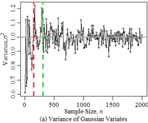
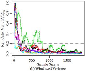
Figure 1. Sample Size vs. Variance Stability. The colours in the right plot denote the distribution: normal, uniform, exponential, Poisson, \(\chi^2\), Student's t, and Birth Rate ABM. - 2.11
- The colours distinguish the seven distributions. The grey,
dashed horizontal line expresses our semi-subjective criterion (of
0.20) under which the relative \(\omega_n^2\) must reside in order for
\(n\) to be deemed a "minimum sample size". The speed at which this
condition is met varies considerably among the distributions,
highlighting the need to forego distributional assumptions regarding
ones ABM outputs in variance-based minimum sample size determination,
unless the distributional shapes are well-identified. This approach for
assessing variance stability bears two elements of further
subjectivity. Firstly, the point of stability may be identified by
either the first \(n\) at which the criterion condition is met or the
first \(n\) at which all further sample sizes meet the condition. The
red and green vertical lines in Figure 1a respectively denote these
points of stability for the Gaussian distribution. Secondly, the outer
variance could have been assessed using a larger pool of variates at
each \(n\) rather than estimated under windows. However, in keeping
with the strategy of minimizing the number of test simulation runs
\(n_{\min}\), we report the findings of window-based \(\omega^2\)
rather than \(\sigma^2\) (\(s^2\)).
Effect Size
- 2.12
- In traditional statistical analysis, the common approach
for determining minimum sample size requires one to first select the
size of a detectable effect (i.e., a statistic such as the mean or
difference of means scaled by a pooled standard deviation). This
approach also requires a selection of acceptable levels of the type
I and type II
errors. A type I error is coarsely the probability (in the frequentist
sense) that the null hypothesis is rejected when in fact it is true.
The type II error is the converse: the likelihood that the null
hypothesis is retained when the alternative hypothesis is true. For
example, one might compare the means of two ABM outcomes each from
separate sets of sample of runs. These outcomes may be borne of distinct
model parameterizations (a necessary though not sufficient condition
for yielding a true difference) and measured to be significantly
different under a rudimentary t-test.
However, a small sample size will penalize the test which may not
report a statistically significant difference between means of those
outcomes: a type II error. Alternatively, these outcomes may arise from
identical parameterizations yet the t-test
erroneously reveals a significant difference: a type I error. The rates
of type I and II errors are expressed as \(\alpha\) and \(\beta\). The
converse of the type II error (\(1-\beta\)) is called the "power"
level.
- 2.13
- The minimum sample size \(n_{\min}\) can then be computed
as
$$ n_{\min} \geq 2 \frac{s^2}{\delta} (t_{V,1-\alpha/2} + t_{V,1-\beta/2})^2 $$ where \(s\) is the standard deviation of the outcome or the pooled standard deviation of two outcomes, \(\delta\) is lower bound on the absolute difference in means that is to be classified as significantly different; \(t\) is the t-statistic (or the quantile function of the t distribution); \(\nu\) is the degrees of freedom (here \(n_{\min} - 1\)), and \(\alpha\) and \(\beta\) are the levels of type I and II errors respectively. In lay terms, the minimum sample size occurs at the point at which both type I and type II errors occur at the desired critical levels as determined by the t-test, hence the employment of the t distribution. This approach has been suggested in the ABM literature (e.g., Radax & Rengs 2010). As \(n_{\min}\) appears on both sides of the equation, trial-and-error or algorithmic iterations can usually converge on \(n_{\min}\). A similar equation is employed when the outcome is a proportion \(\in [0, 1]\). The non-central t distribution can also be used for sample size determination (as in the R statistical package).
- 2.14
- A close inspection of this approach reveals test
sensitivity to the outcome distribution's departure from the
normal. In Table 1, we
empirically measure the power level (and hence the level of type II
error) by drawing pairs of variate sets from some typical distributions
and the Birth Rate model, parameterized such that identical effect sizes
of 0.5.[3]
Thus, an insignificant t-test comparison for a pair
of variate sets is tantamount to a type II error. For each distribution
type and sample size \(n\), the comparison was performed for 5000 pairs
of variate sets each of size \(n\). Each set pair was compared, and we
monitor the proportion of pairs of these sets that yielded a
significant \(p\)-value: an empirically-derived power level. The
empirical power levels for a range of sample sizes \(n\) are
graphically shown in Figures 15
and 16 in Appendix A.
Table 1: Minimum Sample Sizes for Outcome Distributions. \(n_t\), \(n_e\), and \(n_W^{\phantom{x}}\) are the theoretically-derived, empirically-derived, and Wilcox-test-based minimum sample sizes, \(n_{\min}\). Distr. \(n_t\) \(n_e\) \(n_W^{\phantom{x}}\) \(n_e-n_t\) \(n_W^{\phantom{x}}-n_t\) Normal 64 65 68 1 4 Exponential 64 59 78 \(-5\) 14 Poisson 65 61 64 \(-4\) \(-1\) Birth Rate 64 65 70 1 6 Birth Rate (\(d= 1.0\)) 18 19 26 1 8 - 2.15
- We observe incongruities between the theoretical
\(n_{\min}\) (\(n_t\)) and the empirically-derived \(n_e\). In fact,
the power calculation overestimates \(n_{\min}\) for the skewed
distributions (i.e., the exponential and the Poisson). While the
differences in these \(n_{\min}\) are relatively minor, they could have
a material benefit for large scale ABMs for which each run is costly.
However, in these cases, using the t- test for
exposing a predetermined effect size has to be deemed appropriate. For
these surveyed distribution types, the empirical distributions of the
means themselves frequently pass the Shapiro test of normality hence
allowing for the use of the t-test.
- 2.16
- Given the sensitivity of the traditional t-test
to distributional skewness as well as the uncertainty of the
distributional shape in ABM outcomes, one might turn to a more
conservative test, the Wilcoxon ranked sum test
(also known as the Mann-Whitney test);
the \(n_W\) column reports this test's suggested minimum
sample sizes. Interestingly, the more efficient Wilcoxon test appears
to propose a lower minimum size for the Poisson distribution.
- 2.17
- When we assess the efficiency of calculating \(n_{\min}\)
for the Birth Rate ABM, we find that, despite the flatness plus
bimodality of the outcome distribution, the calculation of \(n_{\min}\)
is almost accurate, and the Wilcox test is modestly conservative
compared to the exponential distribution.
Multivariate Stability
- 2.18
- Since most ABMs typically produce multiple outcomes, the
calculation of the required sample size would have to consider all
outcomes of interest. Furthermore, analysis of ABMs often entails an
exploration of parameter settings (or the parameter space) in order to
understand the dependencies between key input parameters and their
outcomes including their variability. Given the complexity of ABMs, the
outcomes' variance may or may not be constant (i.e., homoskedastic)
across the parameter settings. Hence, the task of understanding model
output sensitivity to different experimental conditions that are
relevant to the research question is vital. While the topic of
sensitivity analysis is further elaborated in 3.1, we discuss it here
briefly given its role in determining the adequate run sample size
applicable to all the chosen parameter settings. Well-structured DOE
(described further in Section 3)
can be very helpful to comprehensively explore model variabilities
corresponding to multiple model parameters.
Visualization for statistical issues
- 2.19
- One visualization approach for examining univariate ABM
outcome distributions is the violin plot
which combines elements of a box plot and a kernel density plot, with a
smoothed estimation of outcomes' variances across the ranges of
factors/parameters (see, e.g., Kahl
& Hansen 2015). Figure 2
illustrates the multifaceted influence of six variables (each with 3
values following a \(3^k\) factorial design) on the output measure
("compensation payment"). Details may be found in Lorscheid (2014).

Figure 2. Violin plots for a univariate analysis of potential control variables. Source: Lorscheid (2014) - 2.20
- The grey area indicates the dispersion of values. The white dot in the plot indicates the median of the data set. The black line above the median is the area of the second quartile, and the black line below the median is the third quartile of the data set. For a detailed description of violin plots see Hintze and Nelson (1998).
 Solution space exploration
and sensitivity analysis
- 3.1
- There are a variety of topics that may be gathered under
the broad heading of parameter or input-output space exploration,
including optimization, calibration, uncertainty analysis, sensitivity
analysis, as well as the search for specific qualitative model features
such as "regime shifts" and "tipping points". In all cases, the goal is
to provide additional insight into the behaviour of the ABM through the
examination of certain parameter settings and their corresponding
output measures.
- 3.2
- We will first discuss "exploration" in a broad sense,
followed by a more detailed discussion of a variety of methods for
performing one particularly important exploration task: sensitivity
analysis.
Input/Output Solution Space Exploration
- 3.3
- One of the most common forms of parameter space exploration
is manual (or human-guided)
exploration (also called the
"trial-and-error method" or "educated guessing"). This approach can be
computationally efficient if guided by an individual familiar with the
model's dynamics and/or outputs. The intuitions of a model's
author/developer, a domain expert, or a stakeholder can inform
parsimonious, iterative parameter selection in such a way as to
generate and test relevant hypotheses and minimize the number of
regions searched or the number of required simulation runs. However,
this exploration strategy is vulnerable to human bias and fatigue
leading to a disproportionate amount of attention paid to the target
phenomena and the neglect of large portions of the model's behaviour
space. Distributing the burden of the exploration task (e.g., crowd
sourcing) may address some of its limitations. Nevertheless, more
systematic, automated, and unbiased approaches are required to
complement the shortcomings of solely human-guided searching, which
will always play a role in space exploration, especially in its
preliminary stages.
- 3.4
- The simplest of the systematic exploration approaches fall
under the class of regular sampling techniques
in which the parameters are chosen (or sampled) in a systematic manner
to ensure their having certain statistical or structural properties.
Some of these techniques are random, quasirandom,
gridded/factorial, Latin hypercube,
and sphere-packing. Sampling may globally consider
the entire parameter space or focus locally on a particular region
(e.g., altering one parameter at a time for "univariate sensitivity
analysis"). The well-established methodological history of DOE and the
recent literature on design and analysis of simulation experiments
(e.g., Sacks et al. 1989)
can guide the sampling strategy. However, the complexity of ABMs (and
their outputs) can render classic DOE inappropriate as noted by Sanchez
and Lucas (2002). Classic
DOE (a) assumes only linear or low-order interactions among
experimental parameters (or factors) and outputs, (b) makes little or
no provision for the iterative parameter selection process (i.e.,
sequential virtual experiments), and (c) also assumes typical error
(Gaussian and unimodal) in the output. An example of multi-modal ABM
output is presented in Appendix C. Thus, traditional DOE methods, while
useful for ABMs, ought to be implemented with caution and consideration
for appropriate methods that address complexities in the output.
Research into DOE methods for ABMs is still evolving (Klein et al. 2005; Kleijnen et al. 2005; Ankenman et al. 2008; Lorscheid et al. 2012).
- 3.5
- Research into more sophisticated exploration techniques has
been informed by meta-heuristic searching,
optimization algorithms, and machine
learning. Researchers propose the use of genetic
algorithms (GA) (Holland 1975)
for a wide range of exploration tasks including directed searches for
parameters that yield specific emergent behaviours (Stonedahl & Wilensky 2011),
parameter optimization (Stonedahl
et al. 2010), calibration/parameter estimation (Calvez & Hutzler 2006; Heppenstall et al. 2007; Stonedahl & Rand 2014)
and sensitivity analysis (Stonedahl
& Wilensky 2010). The query-based
model exploration (QBME) paradigm provided by
Stonedahl and Wilensky (2011)
expands Miller's (1998)
application of GA in ABM output exploration. In QBME, parameters
producing user-specified model behaviours are discovered through
automation such as GAs, thus inverting the traditional workflow (see
Figure 3). Stonedahl and
Wilensky (2011)
demonstrate QBME for identifying convergence, divergence, temporal
volatility, and geometric formations in models of collective animal
motion (i.e., flocking/swarming).
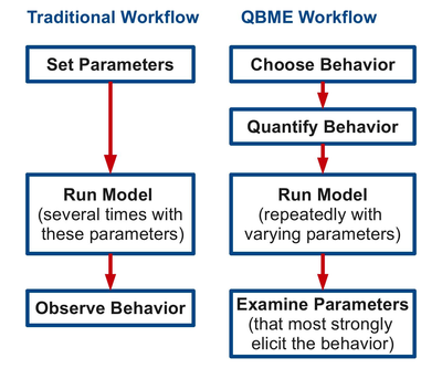
Figure 3. Query-Based Model Exploration (QBME). This framework for exploring ABM parameter-spaces exploits genetic algorithms (or other meta-heuristic search algorithms) to efficiently search for parameters that yield a desired model behaviour. Source: Stonedahl and Wilensky (2011) Sensitivity analysis: Approaches and challenges
- 3.6
- Sensitivity analysis
(SA) is a variation of parameter/input-output space exploration that
focuses on model response to changes in the input parameters (Figure 4). Specifically, the researcher
seeks to identify parameters for which small variations most impact the
model's output.
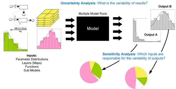
Figure 4. Uncertainty and sensitivity analysis as part of the modelling process. Source: Ligmann-Zielinska et al. (2014) - 3.7
- This discovery can aid in prioritizing prospective data
collection leading to improved model accuracy, reduction of output
variance, and model simplification (Ligmann-Zielinska
et al. 2014). Model insensitive parameters may even be
relegated to mere numerical constants thereby reducing the
dimensionality of the input parameter space and promoting model
parsimony; this simplification process is referred to as "factor
fixing" (Saltelli et al. 2008).
Ignoring these non-influential input parameters can have ill-effects on
the model by increasing its computational cost and also on its
reception when these parameters are controversial for stakeholders not
involved with the model's development (Saltelli
et al. 2008).
- 3.8
- The proliferation of various SA methods stems from the
variety of ABM styles and research problems ABMs address as well as
from the availability of increasing computational capacity (Hamby 1994; Saltelli et al. 2000).
Currently, the ABM practice of SA has entailed one or more of the
following methods: one-parameter-at-a-time, elementary
effects, standardized regression coefficients,
meta-modelling, and variance-based
decomposition (Thiele et
al. 2014; ten Broeke et al.
2014). Below, we briefly discuss each of these, their
advantages, and drawbacks, in the context of ABMs.
- 3.9
- In one-parameter-at-a-time
(OAT), each input parameter in turn is examined over a set of values
(defined either ex ante to the SA or dynamically
during SA) and in isolation by holding the other parameters at a
constant baseline. Meanwhile, the effects of these marginal (i.e.,
one-at-at-time) parameter changes are monitored, and repeated
iterations increase the procedure's robustness. Hassani-Mahmooei and
Parris (2013),
for example, applied OAT to their ABM of micro-level resource conflicts
to identify preferable initial conditions and to evaluate the influence
of stochasticity on the model; the similarity of outcomes within a
threshold demonstrated the model's insensitivity to randomness. OAT's
simplicity while attractive also exposes its limitations in ABM SA (Ligmann- Zielinska 2013). For
one, the impactful and relevant values for each input parameter may be a
priori unknown thus rendering any prioritization of
parameters difficult and the search for key parametric drivers
inefficient. Also, the marginal nature of the parameter search space
surrounding the baseline obscures parameter interactions and severely
shrinks the input hypercube with larger parameter sets. For example,
with as few as 10 input parameters, OAT covers only 0.25% of the input
space (for a geometric proof, see Saltelli and Annoni (2010)).
- 3.10
- Elementary effects
(EE) expands on OAT by relinquishing the strict baseline. That is, a
change to an input parameter is maintained when examining a change to
the next input rather than resuming the baseline value (as done in
OAT). Passing over the parameter set is multiply repeated while
randomly selecting the initial parameter settings. These perturbations
in the entire parameter space classify EE as global SA
(Saltelli et al. 2008).
Originally proposed by Morris (1991)
and improved by Campolongo et al. (2000),
EE is suited for computationally expensive models having large input
sets and can screen for non-influential parameters.
- 3.11
- Global SA may also be performed through estimation of standardized
regression coefficients (SRC), which in its basic
form succinctly measures the main effects of the input parameters
provided the relationships between the parameters and the outcomes are
primarily linear. A standardized regression coefficient
expresses the magnitude and significance of these relationships as well
as the explained variance. More precisely, the square of the
coefficient is the variance explained.
- 3.12
- One glaring limitation of SRC is its ability handle spatial
inputs (of spatial ABMs) unless a small set of scalars or indices can
sufficiently serve as proxies for entire maps (Lilburne & Tarantola 2009).
Also, SRC can expose lower-order effects but not complex
interdependencies (Happe et al. 2006).
- 3.13
- Meta-modelling (or
emulation) can address the low-order limitations of SRC. A meta-model
(emulator, a model of a model) is the surrogate representation of the
more complex model (like ABM) created in order to reduce the
computational time of the simulations necessary for SA. For example, Happe et al. 2006 collated
model responses from a \(2^k\) factorial design on a relatively small
set of parameters and fitted a second-order regression. Meta-modelling
can be computationally efficient and not necessarily require large
amounts of data. For even higher order effects, meta-modelling methods
such as Gaussian process emulators are required (Marrel et al. 2011).
- 3.14
- Variance-based SA
(VBSA) is considered the most prudent approach for evaluating model
sensitivities as it does not assume linearity (Ligmann-Zielinska &
Sun 2010; Fonoberova
et al. 2013; Tang &
Jia 2014). In VBSA, the total variance of a given output is
decomposed and apportioned to the input parameters including their
interactions (Saltelli et al. 2000;
Lilburne & Tarantola
2009). Two indices per input (\(i\)) are drawn from the
partial variances: a first-order (main effects) index \(S_i\) and a
total effects index \(ST_i\). \(S_i\) is the ratio of \(i\)'s partial
variance to the total variance. \(ST_i\) is the sum of all non-\(i\)
indices (\(\sum S_{-i}\)) and captures interactions between \(i\) and
the other inputs (Homma &
Saltelli 1996). \(S_i\) alone is sufficient for decomposing
additive models, so VBSA is unnecessary for models known to produce
largely linear output as calculation of the index pairs is
computationally expensive requiring large sample sizes (Ligmann-Zielinska &
Sun 2010); for example, VBSA for \(k\) parameters requires
\(M\) (\(k+1\)) model runs where \(M>1000\). This computational
load may be reduced through parameter (or factor) grouping (Ligmann-Zielinska 2013;
Ligmann-Zielinska et
al. 2014), parallelization (Tang
& Jia 2014), or quasi-random sampling (Tarantola & Zeitz 2012).
Situations in which inputs are exogenously correlated may result in
non-unique VBSA (Mara &
Tarantola 2012). While recent methods addressing these
dependencies have been developed (Kucherenko
et al. 2012; Mara &
Tarantola 2012; Zuniga et
al. 2013), they still require elaborate DOE coupled with a
very large sample size and algorithmic complexity.
- 3.15
- Genetic algorithms (GAs)
may also be used for SA (Stonedahl
& Wilensky 2010). Parameters are altered under the
genetic paradigm of reproduction in which pairs of "fitter" parameter
sets exchange subsets. The fitness (or objective) function may be
tailored to expose model sensitivities to its parameters (as opposed to
calibration). For example, Stonedahl and Wilensky (2010) allowed GAs to search
through 12 parameters of the "Artificial Anasazi" ABM (Dean et al. 2000; Janssen 2009) in order to
induce responses departing far from the empirical, historical values,
while constraining the search to a limited range (\(\pm\)10% of their
calibrated settings). See Figure 18
in Appendix D for a plot of the outlier results.
- 3.16
- The reliance on mean and variance for distributional
information in many of the practiced methods of SA is insufficient for
more complex distributions. Future research should investigate
moment-independent methods (Borgonovo
2007; Baucells
& Borgonovo 2013).
Visualization in sensitivity analysis
- 3.17
- Visualizations of the input parameter-output relationships
are an integral part of SA. In scatter-plots,
these relationships are directly and simply plotted potentially
revealing dependencies (see Figure 5).
We used the simple Schelling segregation model (Schelling 1969) of red and
green agents on a 100x100 grid implemented in Agent Analyst (http://resources.arcgis.com/en/help/agent-analyst/).
The model contains four uniform parameters (lower and upper bounds in
parentheses): number of agents (3000, 6000; discrete), tolerance to
agents of different colour (0.2, 0.5), random seed (1, 10000; discrete),
and percent of green agents (10, 50). We measured agent migration
(total number of agent moves during model execution) for \(N = 1280\)
model runs.
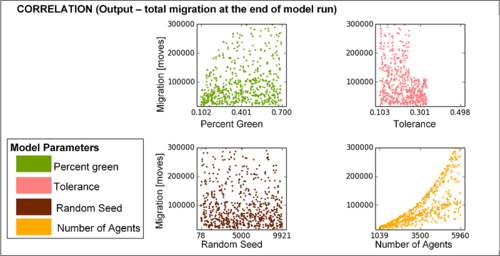
Figure 5. Sensitivity analysis with scatterplots. Scatterplots of total migration versus the four model inputs at \(t = 100\); note that number of agents has more influence on the variability of total agent migration than the other inputs. - 3.18
- Typically, the \(y\)-axis and \(x\)-axis (for a
two-dimensional scatterplot) express values for an output and an input
parameter, respectively. Scatterplots are especially useful when the
dependencies are structured, the output is a scalar, and the number of
model parameters is limited allowing for an unencumbered enumeration of
parameters and output combinations in separate scatterplots. More
complex model behaviours require alternative visualization styles such
as pie charts to display
variance partitions (see Figure 6).

Figure 6. Sensitivity indices obtained from decomposition of migration variance at \(t = 100\). Note that almost 30% of migration variance is caused by interactions among inputs – mainly tolerance and number of agents. - 3.19
- A snapshot of variance decomposition at
the end of the model run (e.g., Figure 6)
may be insufficient in assessing the importance of parameters and
consequently their prioritization (Ligmann-Zielinska
& Sun 2010). Thus, visualizing variance decomposition
temporally will reveal parameter stability over the course of the model
run (see Figure 7). Spatial
outputs such as land use change maps may also receive similar treatment
to reveal the extent of outcome uncertainty in regions (or clusters)
due to specific parameters (Ligmann-Zielinska
2013).
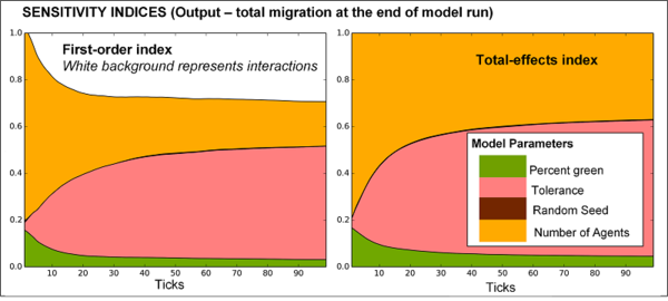
Figure 7. Time series of sensitivity indices obtained from decomposition of migration variance measured over time. The example demonstrates that parameter sensitivities can considerably vary during simulation, with number of agents dominating the variance at \(t = 10\), and tolerance dominating the variance at \(t = 100\). - 3.20
- SA for multiple outcome variables in an ABM incurs additional challenges due to differences in each parameter's impact on the outcomes (see Figure 4). This issue is of particular concern for model simplification and demands either one single, well-chosen outcome that is adequately representative of the model's behaviour or more conservatively, the difficult task of undergoing SA across the whole spectrum of outputs: scalars, time- and space-dependent measures.
 Spatio-Temporal
Dynamics
-
Temporal and spatial dimensions of ABM output data: challenges
- 4.1
- As a stochastic process, an ABM generates (or is capable of
generating) time series (TS) data. To a slightly
lesser extent, ABMs also operate within topological boundaries often
expressed as a spatial landscape, whether empirical (e.g., Parker et al. 2002; Bousquet & Le Page 2004;
Heppenstall et al. 2012;
Filatova 2014) or
stylized (e.g., early use by Schelling
1969, 1978; Epstein & Axtell 1996).
Similar to other ABM outcomes, both the TS and spatial data are borne
out of complex endogenous dynamics over which the modeller exerts full
control. Thus, it is rarely the case that the output data is produced
by a single component of the model. Instead, most of ABM TS and spatial
output recorded embody the long list of unique features that ABMs
exhibit such as emergence rather than aggregation at the macro-level,
interaction rather than reaction at the meso-level, and non-linearity
rather than linearity of processes and decision-making at the
micro-level. Spatial maps generated by ABMs may also capture eventual
spatial externalities, path-dependencies, and temporal lag effects.
These characteristics render the analysis of ABM outputs less
appropriate for more traditional tools. These issues derive from the
reasons ABM are used in the first place.[4]
We consider this challenging nature of TS and spatial output analysis
in the following sections.
Time: approaches and visualization techniques
Time series generated by ABMs (ABM TS) represent a myriad of temporal outcomes, such as evolving agent characteristics (e.g., sociodemographics, utility, opinions); agent behaviours/decisions (e.g., strategies, movements, transformations); or measures descriptive of the model state (e.g., agent population or subpopulation counts). All these are often presented as simple line graphs representing 1) outcomes of individual agents of special interest (Squazzoni & Boero 2002, Fig. 9) or 2) aggregated statistics (such as mean or median) over the entire agent population, subgroups, or an individual (with measurements over several runs) under varying levels of temporal granularity (e.g., a moving window covering several time points) (Izquierdo et al. 2008). Comparisons of multiple TS are often facilitated by the inclusion of confidence intervals (Raczynski 2004, Fig. 4) and occasionally performed against experimental/empirical (Richiardi et al. 2006; Boero et al. 2010, Fig. 1) or theoretical (Takahashi & Terano 2003, Fig. 4) outcomes or expectations (Angus & Hassani-Mahmooei 2015). TS comparisons have also been performed for calibration purposes (Richiardi et al. 2006). - 4.2
- Despite the proliferation of ABMs, effective TS analytical
techniques remain under-used (Grazzini
& Richiardi 2015). Angus and Hassani-Mahmooei (2015) surveyed over 100 ABM
publications in JASSS and found very few instances
of additional
(statistical) modelling of TS data. Only in agent-based financial market
research does one find relevant TS statistical and econometric analysis
(Yamada & Terano 2009;
Chen et al. 2012; Neri 2012).
- 4.3
- In this section, we discuss elements of TS analysis in the
context of ABMs and present some basic and some compelling examples,
while stopping short of expounding formal TS modelling such as
auto-regressive models.
- 4.4
- Among the techniques for analysing ABM TS, we consider time
series decomposition to be one of the more useful
methods. Decomposition entails partitioning a TS into four components:
trend, cyclical, seasonal, and random components. The prominent trend
is the most structured of these components and depicts
the long-term linear or non-linear change in the TS data. The seasonal
component exhibits regular periodicity due to some fixed external cycle
such as seasons, months, weeks, or days of the year. Exogenous model
events such as regular additions of a fixed count of agents to the
agent pool are also considered seasonal. Cycles having irregular
periodicity constitute the cyclical component.
Finally, the residual or random component captures
the unexplained variation remaining after the prior three components
are filtered from the TS.
- 4.5
- The spectrum of TS analysis techniques runs from the
calculation of moving averages
and linear filtering (see
Figures 8a and 8b) to the more
sophisticated exponential smoothing
and autoregressive modelling.
Furthermore, ABM relevant ergodicity tests may be applied to infer
stationarity of statistical moments (e.g., mean, variance, skewness,
kurtosis, etc.) hence equilibrium of those moments across a pool of
simulation runs (Grazzini 2012).
- 4.6
- For an example of ABM TS analysis, we examine the output of
the well-known El-Farol "bar patron" game-theoretic ABM (Rand &
Wilensky 2007). The initial conditions are: memory size = 5, number of
strategies = 10, overcrowding threshold = 50. The number agents
increases by 2% every 52 steps. Figure 8a
presents the original data and its linear increasing trend (in red).
Subtle structure in the TS is exposed when we plot a moving average
along with its decomposed trend (obtained via exponential smoothing)
(Figure 8b).
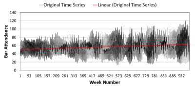
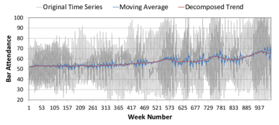
(a) Linear trend (b) Moving average 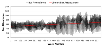
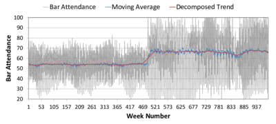
(a) Linear trend (b) Moving average Figure 8. Time Series of Bar Attendance in El Farol ABM. The black and grey series represent the original data; the red line is the linear fit (left) or decomposed trend (right); and the blue line is a moving average. The upper subfigures are labelled (a) and (b). The lower subfigures are (c) and (d). - 4.7
- The model behaviour is augmented to include an arbitrary,
one-time increase in population increase while the gradual increase is
reduced to 0%. While the linear trend for the new results (Figure 8c) coarsely captures the population
increase, the sudden change is made starkly visible using a moving
average (plus decomposed trend) (Figure 8d).
- 4.8
- Comparisons between TS drawn from distinct model
parameterizations can be easily performed through direct (albeit naïve)
visual comparison of the two series, plotting the differences, or
calculating their Euclidean distance[5] or cross
correlation. However, these comparison approaches are applied
to exact temporal pairwise data and thus fail to account for the
complexities of ABMs that may produce TS that are dissimilar only
through interspersed lags. In addition to Richiardi's (2012) suggestions for robust
TS comparison, we advocate the use of dynamic time
warping (DTW) to address the above complication (Keogh & Ratanamahatana 2005).
DTW is now extensively used in areas such as motion and speech
recognition. Using a stylized pair of TS, Figure 9
depicts the effectiveness of DTW, which identifies comparable pairs of
data occurring at differing time scales.

Figure 9. Comparing distance (similarity) measurement methods between Euclidean Distance (left) and DTW (right) - 4.9
- To further demonstrate DTW's effectiveness, we compare 40
distinct parameter settings in Epstein's ABM of civil violence (Epstein 2002; Wilensky 2004).
The primary
distinction is the initial cop density which ranges from 4.05 and 5.00
in increments of 0.05% and results in varied sizes of the population of
quiet citizens, our outcome measure of interest here. We obtain 10 TS
samples (i.e., model runs) under NetLogo each having a duration of 200
ticks/time points. In Figure 10,
we present four individual runs in order to highlight the difficulty of
direct visual comparison.
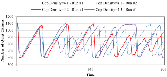
Figure 10. Comparing Time Series from Distinct Parameterizations of Quiet Citizens of Civil Violence ABM - 4.10
- While the outcomes are initially similar, they rapidly
diverge sharing only the characteristic of the outcomes' exhibiting
some fluctuation. The two runs under the same parameter setting (4.1%)
naturally diverge due to distinct random sequences (from a RNG using
distinct random seeds).
- 4.11
- Comparisons of all pairs of the experimental conditions are
presented in Figure 11. These
comparisons are performed on normalized outcomes averaged over the
suite of runs. The distance measurements in the left matrix are direct
correlations and Euclidean distances in the right matrix. The cells in
the upper triangle of each matrix correspond to direct comparison of
the TS while those in the lower triangle indicates the measurements
under DTW. The row and columns denote increasing cop densities.
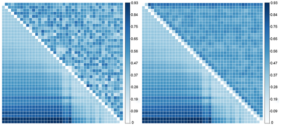
Figure 11. Comparing DTW against non-DTW for correlation and Euclidean distance - 4.12
- The figures illustrate the superiority of DTW in capturing
TS differences under these measurements, over the direct use of exact
temporal pairs. DTW clearly exposes greater similarity of the outcomes'
TS when the experimental parameters (cop density) are also similar
whereas the direct measurements do not. This relationship is largely
monotonic as one would expect. Thus, DTW is appropriate for models for
which the outcome TS's structure (specifically, both its seasonal and
irregular periodicities) is greatly affected by the experimental
conditions.
- 4.13
- Finally, TS analysis provides a highly informative
opportunity to precisely estimate the impact of changes in the input
variables on the outputs of an ABM model. Techniques such as panel
data (or longitudinal)
analysis, which take into account both TS and cross sectional
components of the data, can enable the agent-based modellers to uncover
robust evidence on how model behaviours are associated with the changes
in the variables of the agents and/or the model over time. Other
prominent components of TS analysis (such as forecasting,
classification and clustering,
impulse response function, structural
break analysis, lag analysis,
and segmentation) may also be
used along with estimation and auto-regressive methods in order to
provide a better understanding of series generated by ABMs.
Processing spatial ABM output: approaches and visualization techniques
- 4.14
- The spatial environment in ABMs vary from cellular grids
(in which only inter-agent distance matter) to raster or vector
representations of multiple layers of a rich GIS data. Locations in a
spatial ABM may relate to output metrics at the individual or
aggregated agent level (e.g., income, opinion, or a strategy) or other
spatial qualities (e.g., land-use categories). It is challenging to
seek patterns and to compare across experimental conditions
in a search for a compelling narrative while screening through hundreds
of maps produced by an ABM. Spatial ABM analysis is often informed by
methods from geography and spatial statistics/econometrics. Here, we
review some spatial metrics and visualization approaches for spatial
analysis.
- 4.15
- Quantitative indices such as the Kappa
index of agreement (KIA or Cohen's \(\kappa\)) have
been widely employed for cell-by-cell comparison of ABM outcomes on
spatial maps (Manson 2005).
More recent work suggest alternatives to the \(\kappa\) such as a moving
window algorithm (Kuhnert
et al. 2005) and expose its limitations (Pontius & Millones 2011).
Pontius (2002) proposes
more comprehensive methods and measures for tracking land use changes
and comparing maps under multiple resolutions (from coarse to fine).
- 4.16
- Various spatial metrics
are often used to measure land-use change and detect spatial patterns
such as fragmentation and sprawl (Parker
& Meretsky 2004; Torrens
2006; Liu & Feng 2012;
Sun et al. 2014). These
metrics include mere counting of land-use categories, landscape
shape index, fractal dimension, edge
density, as well as adjacency, contiguity,
and centrality indexes. Moran's I
is another spatial autocorrelation statistic indicating the extent of
dispersion or clustering (Wu 2002).
Millington et al. (2008)
used a contagion index along
with basic patch count metrics to identify fragmentation. Griffith et
al. (2010) used Getis-Ord
Gi* "hotspot" analysis to identify statistically significant
spatial clustering of high/low values while analysing the spatial
patterns of hominids' nesting sites. Zinck and Grimm (2008) used spatial indices (shape
index, edge index ) and basic metrics
(counts and areas of discrete "island" regions) to systematically
compare empirical data to simulation results from the classic
Drossel-Schwabl forest fire cellular automata ABM. Software offering
these metrics include C++ Windows-based 'FRAGSTATS' and the 'SDMTools'
package (for the platform-independent R), the functionality of which
may be augmented by Bio7 and ImageJ for image processing.
- 4.17
- In another example, Sun et al. (2014,
Table 6) reported basic statistics (i.e., mean and standard deviation)
on nine spatial metrics estimated over multiple parameter settings for
varying levels of land market representation in their urban ABM. The
significance of mean differences (across conditions) were assessed with
the Wilcoxon signed rank test.
Means of the metrics were jointly visualized across all parameter
settings in a line graph style called "comprehensive plotting" (Sun et al. 2014, Figures 5–8),
which then allows for identification of conditions producing outlying behaviour facilitating visual sensitivity analysis.
- 4.18
- Obviously, statistical models such as regressions and
ANOVAs may be employed to relate model parameters and outcomes to
spatial outcomes (e.g., Filatova
et al. 2011). However, dependencies among spatially
distributed variables require special treatment in the form of a
weighted matrix incorporated into a spatial
regression model as a predictor or as part of the
error term. Locales may be disambiguated further in statistical
prediction through geographically weighted regression
(GWR). These methods also fall under the auspices of spatial
econometrics.
Reporting and visualizing ABM results over time and space
- 4.19
- Typically, spatial ABM output is rendered as
two-dimensional maps. A collection of these can highlight model
dynamism/progression or allow for comparison of metrics and
experimental conditions (Parry
& Bithell 2012, Figure 14.11) or expose key,
informative trajectories (e.g., Barros
2012, Figure 28.3). 3D views are also used to portray outputs
particularly in evacuation and commuting (Patel
& Hudson-Smith 2012). Often, visual inspection of the
data offers face validation and high-level inference. For example, a spatial
overlay is commonly used to analyse raster outputs
and evaluate the spatial distribution of multiple model behaviours and
outcomes.
- 4.20
- The spatial distribution of outcomes is subject to the
stochastic and path dependent nature of ABMs and often demand
aggregation for effective presentation of model behaviour (Brown et al. 2005). Naturally, a
mean with a confidence interval for an outcome in each spatial location
can be sufficient for reporting a set of maps (over time or across
experimental conditions) (e.g., Tamene
et al. 2014). Alternatively, a frequency
map for a single parameter setting reveals each
location's state transition probabilities (as a proportion of total
simulation runs) (Brown et al. 2005).
These transitions may easily be portrayed as a colour-gradient
map (e.g., Magliocca
2012). Plantinga and Lewis (2014)
warn against constructing deterministic transition rules out of these
probabilities. Brown et al. (2005)
also suggest distinguishing areas of non-transition (or invariant
regions) from variant regions; the method for identifying these areas
is called the variant-invariant method.
- 4.21
- Judicious selection of a temporal sequence of maps can
reveal model dynamics. Software such as a "map comparison kit" (RIKS BV 2010) can perform
automated tests to identify the extent to which two raster maps are
different. Pontius et al. (2008)
extends the comparison exercise to include three maps while considering
pixel error and location error. Comparisons include all pairs of
simulation outputs at times 1 and 2, a "true", reference map at time 2,
and all three maps jointly.
- 4.22
- While showcasing a map as an output of an ABM is always
appealing, supplementing it with summary statistics of spatial patterns
allows for deeper understanding of experimental effects and
consequently the model's behaviour. In addition to the spatial metrics
discussed in 4.3, quantities of land use and conversions may be
reported as histograms across different scenarios and land-use types
over time (e.g., Figure 4 in Villamor et al. (2014)).
- 4.23
- Color-gradients in landscape visualizations can be used to
represent temporal changes in a metric of interest. Filatova (2014) employs these spatio-temporal
change gradients to present land price changes
(due to market trades in an ABM focusing on coastal properties) between
two points in time in an empirical landscape (Figure 12).
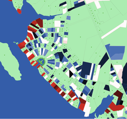
Figure 12. Changes in property prices over time - 4.24
- The blue and red gradients correspond to the valence of the
change (i.e., falling and rising prices, respectively); their darkness
or intensity indicate level of change. Such visualizations may offer
easy identification of clusters and boundaries.
- 4.25
- Another obvious way to depict the differences in spatially
distributed ABM output data is to visualize in 3D plots. The 3rd
dimension clearly permits the inclusion of additional information such
as time or one of agents' inner attributes. For example, Huang et al. (2013) employed 3D colored bar
plots (Figure 13) in which the
2D layout corresponds to physical location.
- 4.26
- Such 3D visualizations offer insights into the ABM's
dynamics or highlight vital structural differences across experiments.
For example, Dearden and Wilson (2012)
use a 3D surface to plot the macro metrics of interest of their retail
ABM as a function of different values of the two most critical
parameters affecting agents' choices. 3D surfaces over different
parameters spaces can also be compared with each other, as demonstrated
by Dearden and Wilson in their comparisons of activity within consumer
and retailer agent classes.
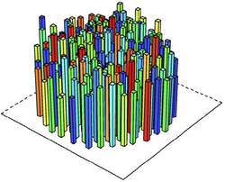
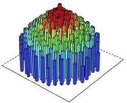
Figure 13. Price of land and sequence of transactions under various market conditions when agents have heterogeneous preferences for location. Left: Allocation of land on this market is only preference driven. Right: Land allocation happens through competitive bidding. The higher the bar, the higher the land price. colours denote the time when land was converted into urban use. Source: Huang et al. (2013) - 4.27
- In this example, the color adds a fourth dimension (time of
an event) to the conveyed information. Furthermore, functional shapes
are more easily discernible in 3D; in this case, the upper section of
Figure 13b might be fitted to
a paraboloid or a similar solid of revolution.
- 4.28
- Another efficient use of 3D visualization for ABMs with
geo-spatial elements is shown in Figure 14.
Malleson's model of burglary in the context of urban
renewal/regeneration comprises agents who travel to commit crime in an
urban landscape (Malleson et al.
2013).
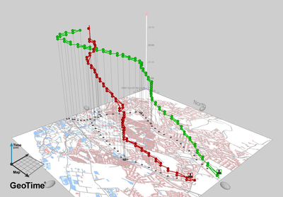
Figure 14. Spatio-temporal Trajectories of Burglars. Source: Nicolas Malleson. http://nickmalleson.co.uk/research - 4.29
- The colored, segmented lines in the figure when overlaid
onto the 2D city map depict the
trajectories of burglar agents seeking targets while the z-axis
denotes the temporal dimension to their journey.
This joint portrayal of time and space succinctly communicates
important features such as key locations of activity for the agents
(i.e., where lines appear vertical) as well as the origin of the agent
and its destination, in this case a presumably "safe" location.
- 4.30
- Finally, given the dynamic nature of ABMs, their spatial and temporal outputs are appropriate for dynamic presentation modalities. Interactive 3D visualizations offer the ability to examine the data from alternative perspectives. Increasingly, video (or animation) has been used to capture ABM behaviour as a means to communicate ABM output to both practitioners as well as the broader lay-audience.[6] Model behaviour may also be captured as animated GIF files, the small sizes of which facilitate their use in presentations and web pages (Lee & Carley 2004; Lee 2004).
 Discussion
and conclusions
- 5.1
- While ABM as a technique offers many exciting opportunities
to open research frontiers across a range of disciplines, there are a
number of issues that requires rigorous attention when dealing with ABM
output data. This paper highlights the outstanding complexities in the
ABM output data analysis and consolidates currently-used techniques to
tackle these challenges. In particular, we group them into 3 themes:
(i) Statistical issues related to defining the
number of appropriate runs and hypothesis testing,
(ii) Solution space exploration and sensitivity
analysis, and (iii) Processing
ABM output data over time and space. We also
briefly discuss stakeholder involvement in ABM
research (iv) below.
- 5.2
- Statistical issues related to defining a number of
runs and hypothesis testing: For analysing ABMs, the
calculation of statistics from model outcomes across multiple
simulation runs is required. However, the statistical methods are
challenged by both a plethora of ABM output data for which traditional
statistical tests will expose minute effects and complex ABMs for which
runs are costly. In the former scenario, statistical methods need to be
tempered (e.g., a more critical \(p\)-value) or an acceptable ceiling
on the number samples (or runs) should be enforced. For the latter
case, a predetermination of test sensitivity (e.g., effect size) must
be made before calculating a minimum number of runs. However, the
stability of outcome variance needs to be secured, and we demonstrate
and review approaches for estimating the point at which this is
achieved. We also reveal that the traditional approach to determining
minimum sample size is sensitive to the shape of the distribution and
we suggest empirical estimation of the power level or use of the more
conservative Wilcoxon rank sum test. Another challenge is the analysis
of many influencing variables. The analysis of complex
interdependencies within a simulation model can be addressed by
systematic design of experiment principles, and univariate analysis may
support the analysis by pre-defining parameter ranges. Overall, ABM
researchers should be aware of the statistical pitfalls in the analysis
of simulation models and of the methods described to address these
challenges.
- 5.3
- Solution space exploration and sensitivity analysis:
An ABM cannot be properly understood without exploring the range of
behaviours exhibited under different parameter settings and the
variation of model output measures stemming from both random and
parametric variation. Accordingly, it is important for ABM analysts and
researchers to be familiar with the range of methods and tools at their
disposal for exploring the solution space of a model, and for
determining how sensitive model outputs are to different input
variables. ABMs pose particular challenges for SA, due to the
nonlinearity of interactions, the non-normality of output
distributions, and the strength of higher-order effects and variable
interdependence. While some model analyses may find success using
simple/classic SA techniques, practitioners would do well to learn
about some of the newer and more sophisticated approaches that have
been (and are being) developed in an effort to better serve the ABM
community.
- 5.4
- Processing ABM output data over time and space:
While every ABM has the potential to produce high resolution panel data
on aggregated and agent-level metrics over long time periods, the
standard time series techniques are rarely applied. We argue that the
use of time series techniques such as decomposition and moving averages
analysis not only improve the scientific value of ABM results but also
help gaining valuable insights – e.g., the emergence of the two regimes
in the data over time – that are likely to be omitted otherwise. The
use of Euclidean distance similarity measurement and dynamic time
warping offers high utility especially when temporally varying outputs
need to be compared between experiments or in a sensitivity analysis
exercise. When dealing with spatial data analysis, ABM researchers
actively use methods developed in geography such as spatial indexes,
map comparison techniques, series of 2D or 3D maps, 2D histograms, and
videos. In addition, ABM-specific methods are being actively proposed –
such as 3D histograms reflecting temporal changes over a spatial
landscape, spatio-temporal output variable change gradients, as well as
overlaying temporal ABM dynamics over a 2D map.
- 5.5
- Communicating ABM results to stakeholders:
The utility and effectiveness of many ABMs and their outputs are often
judged by the model's consumers: the user, the stakeholder, or
decision-maker. Thus, a qualitative understanding of the model is
essential as model acceptance and adoption depend strongly on
subjective, qualitative considerations (Bennett
et al. 2013).
- 5.6
- The clarity and transparency of ABM mechanisms facilitate
stakeholder involvement in the modelling process. This participatory
modelling is a powerful strategy to facilitate decision-making,
management, and consensus building (Voinov
& Bousquet 2010).
In contrast to other techniques
such as System Dynamics (SD), Computational General Equilibrium, or
Integrated Assessment Modelling, ABM rules are explicit, directly
embedded in the model, and do not necessarily have to be aggregated or
proxied by obscure equations. Thus, ABMs have been historically at the
forefront of participatory modelling. Communicative graphical user
interfaces (GUIs) in platforms such as NetLogo and Cormas have also
contributed to the clarity in presentation and ease of interpretation
(as they have done for SD's Stella or Vensim). A clone of participatory
modelling with ABMs conceived by French modellers became known as companion modelling (Bousquet et
al. 1999; Barreteau et
al. 2003; Étienne 2014)
and is applied globally particularly in developing nations (Becu et al. 2003; Campo et al. 2010; Worrapimphong et al. 2010).
As the focus is on the model as a process rather than a product (Voinov & Bousquet 2010),
co-learning between stakeholders and modellers results in expedient
cycles of modelling, output presentation and discussion, and subsequent
amendment of the model.
- 5.7
- Moss (2008)
notes that evidence should precede theory, whenever modelling becomes
embedded in a stakeholder process. Thus, interpretation of model
outputs requires more than mere quantitative evaluation and
interpretation, and the necessary task of weighing model outputs
against values and perceptions of both stakeholders and modellers alike
continues to challenge us (Voinov et
al. 2014).
- 5.8
- Directions for future research: Most of the challenges and techniques considered in this paper are quite computationally intensive. Yet, the fact that an analysis of ABM output data often requires more time and attention than the design and coding of an ABM itself is still largely underestimated especially by amateurs in the ABM field. Thus, user-friendly software products that support design of experiments (e.g., the AlgDesign package in R (Wheeler 2011)),[7] parameter space exploration, sensitivity analysis, temporal and spatial data exploration are in high demand. For example, the MEME software is one step toward this goal and is a valuable tools for ABM researchers. ABMs would ideally support real world decision-making, hence efficient, user-friendly ABM platforms, supporting data analysis and visualization, would reinforce use of ABM in participatory modelling. Moreover, insights into advanced statistical techniques could assist in resolving some of the statistical issues discussed in Section 2.
 Acknowledgements
- This material is based upon work supported by NWO DID MIRACLE (640-006-012), NWO VENI grant (451-11-033), and EU FP7 COMPLEX (308601). Furthermore, our thanks go to all participants of Workshop G2 during the iEMSs 2014 Conference in San Diego.
 Notes
Notes
-
1This
paper was inspired by a workshop at the 2014 iEMSs conference: the G2
workshop "Analyzing and Synthesizing Results from Complex
Socio-ecosystem Models with High-dimensional Input, Parameter, and
Output Spaces". During that workshop, several key issues facing today's
simulation modellers were identified and discussed. The ones deemed to
be more exigent have become the focus of this paper.
2The normal or Gaussian distribution also known as the "bell-curve" is the most easily recognized empirical distribution containing a single mode and often captures many naturally observed outcomes. The uniform distribution is a flat, artificial distribution and can be considered to serve as the control distribution among this set. The exponential is often used to model failure rates and is amodal and skewed. The Poisson expresses the probability of a given number events occurring within a known interval. The \(\chi^2\) (chi-squared) is typically employed in statistical tests as well as the Student's t distribution. We include these two as they are readily recognizable by many practitioners of applied statistics.
3The effect size calculation we employ is Cohen's \(d\) (Cohen 1988): \(d = \frac{\mu_1 - \mu_2}{s_{\rm pooled}}\).
4LeBaron et al. (1999, p. 1512), for example, note that their artificial stock market has time series capturing phenomena observed in real markets, including weak forecastability and volatility persistence.
$$ \mathrm{Euclidean~distance} = \sqrt{\sum^{n}_{i=1} (x_i - y_i)^2} $$ where \(n\) is the number of data points in each vector.
6For examples, we cite Epstein & Axtell (1996) and the corresponding video: https://www.youtube.com/watch?v=SAXWoRcT4NM and Helbing et al. (2005) and the corresponding video: https://www.youtube.com/watch?v=yW33pPius8E.
7Further options in R for DOE may be found at http://cran.r-project.org/web/views/ExperimentalDesign.html.
 Appendix
A: Minimum Sample Size for Distributions
-
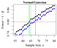
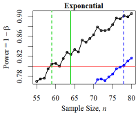
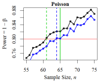
Figure 15. Minimum Sample Size for Three Distributions The black curve denotes the empirical power level. The red line denotes the desired power level: \(1 - \beta = 0.80\). The solid green vertical line denotes the minimum sample size derived from the power calculation while the dotted green line shows the empirically-derived size. The blue curve and line denote the power and minimum size according to the two sample Mann-Whitney-Wilcoxon test.
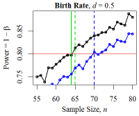
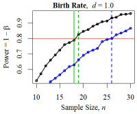
Figure 16. Minimum Sample Sizes for Birth Rate ABM The red line denotes the desired power level: \(1 - \beta = 0.80\). The solid green vertical line denotes the minimum sample size from the power calculation; the dotted green line shows the empirically- derived size; and the blue curve and vertical line denote the power and minimum sample size according to the Mann-Whitney-Wilcoxon test.
 Appendix
B: Issues of Hypothesis Testing
- There exists an ongoing debate over the emphasis researchers should place on significance tests. A large sample size can easily classify a minute difference as being significant. Thus, many (in the ABM field and outside) argue for greater attention paid towards the effect size itself (whether it is Cohen's d or a standardized regression coefficient) as the benchmark for a "significant" finding (Coe 2002; Ziliak & McCloskey 2008, 2009; Sullivan & Feinn 2012; White et al. 2013; Troitzsch 2014). In fact, recently the journal of Basic and Applied Social Psychology has implemented policy to remove \(p\)-values from their publications. Alternatively, researchers may turn to methods and measures that penalize (or minimize the impact of) large samples sizes. Rouder et al. (2009) demonstrate the effectiveness of such penalties in measures such as the Bayesian information criterion and the JSZ Bayes factor. Cameron and Trivedi (2005, p.279) suggest using \(\sqrt{\log n}\) as a more stringent, critical t-statistic. An earlier suggestion by Good (1982, 1984, 1992) entails adjusting the critical p-value using a sample size of \(n = 100\) as a reference point rather than leaving it fixed (e.g., \(p < 0.05\)) for all sample sizes. Furthermore, the estimated minimum sample size may be reduced through variance reduction by control variates which are outcomes having known mean and variance and are sufficiently correlated with other outcomes of interest for which the mean and variance are unknown. This technique is discussed in the context of simulation models by Law and Kelton (2007). Finally, sample size determination for large simulations which are costly to run (i.e., demanding heavy computing resources and incurring long execution times) may be addressed through bootstrapping of a smaller set of outcomes for estimating their variance (Lee & Carley 2013).
 Appendix
C: Multi-Modal ABM Output of Birth Rate ABM
-
Multi-modality in the output may indicate separate attractors in the
phase space bridged by tipping points. For example, the output
distribution (a subpopulation) of a simple, population genetics ABM (Wilensky 1997, 1999) under a single
parameter setting exhibits clear bimodality (Figure 17).
The carrying capacity was set to 200; the fertility rate for both red
and blue populations was 2.0; and 10000 runs of 300 steps were
performed.
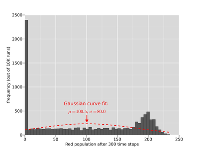
Figure 17. Birth Rate ABM Output Distribution. Histogram of the "red" population after 300 times steps, fitted to a Gaussian curve (from the NetLogo Simple Birth Rates Model (Wilensky 1997)) Interpreting the mean red agent population of 100.5 (with a large degree of error) as being singularly and truly descriptive of the stochastic process would be grossly inaccurate and overlook the salient bifurcation in which the red agent population tends to either diminish to extinction (0) or dominate (around 200). This example illustrates how ABM stochasticity may produce non-normally distributed output that cannot be sensibly described by merely its mean and variance.
 Appendix
D: Anasazi Model Outliers
-
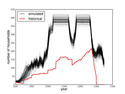
Figure 18. Sensitivity analysis example. Source: Stonedahl and Wilensky (2010) The red line denotes the historical data and the black lines represent outcomes from 100 simulated runs parameterized (via a GA search) to produce output time-series that maximally differ from the historical data.
 References
- ABRAHAMSON, D., Blikstein,
P. & Wilensky, U. (2007). Classroom model, model classroom:
Computer-supported methodology for investigating collaborative-learning
pedagogy. Proceedings of the Computer Supported Collaborative
Learning (CSCL) Conference, 8(1), 46–55. [doi:10.3115/1599600.1599607]
AN, G. & Wilensky, U. (2009). From artificial life to in silico medicine: Netlogo as a means of translational knowledge representation in biomedical research. In: Artificial life models in software (Adamatzky, A. & Komosinski, M., eds.). Berlin: Springer-Verlag.
ANGUS, S. D. & Hassani-Mahmooei, B. (2015). "Anarchy" Reigns: A Quantitative Analysis of Agent-Based Modelling Publication Practices in JASSS, 2001-2012. Journal of Artificial Societies and Social Simulation, 18(4), 16 https://www.jasss.org/18/4/16.html
ANKENMAN, B., Nelson, B. L., & Staum, J. (2008). Stochastic kriging for simulation metamodelling. In: Proceedings of the 40th Conference on Winter Simulation. Winter Simulation Conference, pp. 362–370.
AXELROD, R. & Hammond, R. A. (2003). The evolution of ethnocentric behaviour. In: Midwest Political Science Convention, Chicago, IL.
AXTELL, R. L., Epstein, J. S., J. M. andf Dean, Gumerman, G. J., Swedlund, A. C., Harburger, J., Chakravartya, S., Hammond, R., Parker, J. & Parker, M. (2002). Population growth and collapse in a multiagent model of the Kayenta Anasazi in long house valley. In: Proceedings of the National Academy of Sciences, vol. 99 (suppl 3), 7275–7279. [doi:10.1073/pnas.092080799]
BARRETEAU, O. et al. (2003). Our companion modelling approach. Journal of Artificial Societies and Social Simulation 6(2), 1. https://www.jasss.org/6/2/1.html.
BARROS, J. (2012). Exploring urban dynamics in latin american cities using an agent-based simulation approach. In: Agent-Based Models of Geographical Systems (Heppenstall, A. J., Crooks, A. T., See, L. M. & Batty, M., eds.). Netherlands: Springer, pp. 571–589. .
BAUCELLS, M. & Borgonovo, E. (2013). Invariant probabilistic sensitivity analysis. Management Science, 59(11), 2536–2549. [doi:10.1287/mnsc.2013.1719]
BECU, N., Perez, P., Walker, A., Barreteau, O. & Le Page, C. (2003). Agent based simulation of a small catchment water management in northern Thailand: Description of the CATCHSCAPE model. Ecological Modelling, 170(2–3), 319–331. [doi:10.1016/S0304-3800(03)00236-9]
BENNETT, N., Croke, B., Guariso, G., Guillaume, J. H., Hamilton, S. H., Jakeman, J. & Marsili-Libelli, S. (2013). Characterising performance of environmental models. Environmental Modelling & Software, 40, 1–20. http://www.sciencedirect.com/science/article/pii/S1364815212002435. [doi:10.1016/j.envsoft.2012.09.011]
BOERO, R., Bravo, G., Castellani, M. & Squazzoni, F. (2010). Why bother with what others tell you? An experimental data-driven agent-based model. Journal of Artificial Societies and Social Simulation, 13(3), 6. https://www.jasss.org/13/3/6.html
BORGONOVO, E. (2007). A new uncertainty importance measure. Reliability Engineering & System Safety, 92(6), 771–784. [doi:10.1016/j.ress.2006.04.015]
BOUSQUET, F., Barreteau, O., Le Page, C., Mullon, C. & Weber, J. (1999). An environmental modelling approach: The use of multiagent simulations. In: Advances in environmental and ecological modelling (Blasco, F., ed.). Paris: Elsevier, pp. 113–122.
BOUSQUET, F. & Le Page, C. (2004). Multi-agent simulations and ecosystem management: a review. Ecological modelling, 176, 313–332. [doi:10.1016/j.ecolmodel.2004.01.011]
BROWN, D. G., Page, S., Riolo, R., Zellner, M. & Rand, W. (2005). Path dependence and the validation of agent-based spatial models of land use. International Journal of Geographical Information Science, 19(2), 153–174. . [doi:10.1080/13658810410001713399]
BROWN, D. G. & Robinson, D. T. (2006). Effects of heterogeneity in residential preferences on an agent-based model of urban sprawl. Ecology and Society, 11(1).
BRYSON, J. J., Ando, Y. & Lehmann, H. (2007). Agent-based modelling as scientific method: A case study analysing primate social behaviour. Philosophical Transactions of the Royal Society B: Biological Sciences, 362(1485), 1685–1698.
CALVEZ, B. & Hutzler, G. (2006). Automatic tuning of agent-based models using genetic algorithms. In: Multi-Agent Based Simulation VI, Lecture Notes in Computer Science (Sichman, J. & Antunes, L., eds.). Berlin/Heidelberg: Springer, pp. 41–57.
CAMERON, A. C. & Trivedi, P. K. (2005). Microeconomics: Methods and Applications. Cambridge: Cambridge University Press.
CAMPO, P., Bousquet, F. & Villanueva, T. (2010). Modelling with stakeholders within a development project. Environmental Modelling & Software, 25(11), 1302–1321. http://www.sciencedirect.com/science/article/pii/S1364815210000162. [doi:10.1016/j.envsoft.2010.01.005]
CAMPOLONGO, F., Kleijnen, J. & Andres, T. (2000). Screening methods. In: Sensitivity Analysis (Saltelli, A., Chan, K. & Scott, E. M., eds.). UK: Chichester: Wiley-Interscience, pp. 65–80.
CARLEY, K., Fridsma, D., Casman, E., Yahja, A., Altman, N., Chen, L., Kaminsky, B. & Nave, D. (2006). Biowar: Scalable agent-based model of bioattacks. IEEE Transactions on Systems, Man and Cybernetics, Part A, 36(2), 252–265. [doi:10.1109/TSMCA.2005.851291]
CARLEY, K. M. & Lee, J.-S. (1998). Dynamic organizations: Organizational adaptation in a changing environment. In: Advances in Strategic Management: Disciplinary Roots of Strategic Management, vol. 15. Greenwich, CT: JAI Press, pp. 269–297.
CHANG, M.-H. & Harrington, J.E. (2006). Agent-based models of organizations. In: Handbook of computational economics volume 2: Agent-based computational economics (Tesfatsion, L. & Judd, K. L., eds.). Amsterdam: Elsevier B.V., pp. 949–1011.
CHEN, S.-H., Chang, C.-L. & Du, Y.-R. (2012). Agent-based economic models and econometrics. The Knowledge Engineering Review, 27(2), 187–219. [doi:10.1017/S0269888912000136]
COE, R. (2002). It's the effect size, stupid: What effect size is and why it is important. In: Annual Conference of the British Educational Research Association. University of Exeter, England.
COHEN, J. (1988). Statistical Power Analysis for the behavioural Sciences. Lawrence Erlbaum Associates.
CONTINI, B., Leombruni, R. & Richiardi, M. (2007). Exploring a new expace: The complementarities between experimental economics and agent-based computational economics. Journal of Social Complexity, 3(1), 13–22.
DEAN, J. S., Gumerman, G. J., Epstein, J. M., Axtell, R. L., Swedlund, A. C., Parker, M. T. & McCarroll, S. (2000). Understanding Anasazi culture change through agent-based modelling. In: Dynamics in human and primate societies: Agent-based modelling of social and spatial processes (Kohler, T. & Gumerman, G., eds.). Oxford, UK: Oxford University Press, pp. 179–205.
DEARDEN, J. & Wilson, A. (2012). The relationship of dynamic entropy maximising and agent-based approaches in urban modelling. In: Agent-Based Models of Geographical Systems (Heppenstall, A. J., Crooks, A. T., See, L. M. & Batty, M., eds.). Springer Netherlands, pp. 705–720. .
DUFFY, J. (2006). Agent-based models and human subject experiments. In: Handbook of computational economics volume 2: Agent-based computational economics (Tesfatsion, L. & Judd, K. L., eds.). Amsterdam: Elsevier B.V., pp. 949–1011.
EFFKEN, J. A., Carley, K. M., Lee, J.-S., Brewer, B. B. & Verran, J. A. (2012). Simulating Nursing Unit Performance with OrgAhead: Strengths and Challenges. Computers Informatics Nursing, 30(11), 620–626. [doi:10.1097/NXN.0b013e318261f1bb]
EPSTEIN, J. M. (2002). modelling civil violence: An agent-based computational approach. Proceedings of the National Academy of Sciences of the United States of America, 99(Suppl 3), 7243–7250. [doi:10.1073/pnas.092080199]
EPSTEIN, J. M. & Axtell, R. (1996). Growing artificial societies: Social science from the bottom up. Washington, DC: Brookings Institution Press.
ÉTIENNE, M. (2014). Companion Modelling. Springer. http://link.springer.com/10.1007/978-94-017-8557-0. [doi:10.1007/978-94-017-8557-0]
FILATOVA, T. (2014). Empirical agent-based land market: Integrating adaptive economic behaviour in urban land-use models. Computers, Environment and Urban Systems http://www.sciencedirect.com/science/article/pii/S0198971514000714.
FILATOVA, T., Parker, D. C. & van der Veen, A. (2011). The Implications of Skewed Risk Perception for a Dutch Coastal Land Market: Insights from an Agent-Based Computational Economics Model. Agricultural and Resource Economics Review, 40(3), 405–423. http://ideas.repec.org/a/ags/arerjl/120639.html.
FISHER, R. A. (1971). The Design of Experiments. Hafner.
FONOBEROVA, M., Fonoberov, V. A. & Mexic, I. (2013). Global sensitivity/uncertainty analysis for agent-based models. Reliability Engineering & System Safety, 118(0), 8–17. [doi:10.1016/j.ress.2013.04.004]
GHORBANI, A., Bots, P., Dignum, V. & Dijkema, G. (2013). Maia: A framework for developing agent-based social simulations. Journal of Artificial Societies and Social Simulation, 16(2), 9. https://www.jasss.org/16/2/9.html
GOOD, I. J. (1982). Standardized tail-area probabilities. Journal of Statistical Computation and Simulation, 16, 65–66. [doi:10.1080/00949658208810607]
GOOD, I. J. (1984). C191. how should tail-area probabilities be standardized for sample size in unpaired comparisons? Journal of Statistical Computation and Simulation, 19(2), 174–174.
GOOD, I. J. (1992). The Bayes/non-Bayes compromise: A brief review. Journal of the American Statistical Association, 87(419), 597–606. [doi:10.1080/01621459.1992.10475256]
GRAZZINI, J. (2012). Analysis of the emergent properties: Stationarity and ergodicity. Journal of Artificial Societies and Social Simulation, 15(2), 7. https://www.jasss.org/15/2/7.html
GRAZZINI, J. & Richiardi, M. (2015). Estimation of ergodic agent-based models by simulated minimum distance. Journal of Economic Dynamics and Control, 51, 148–165. [doi:10.1016/j.jedc.2014.10.006]
GRIFFITH, C. S., Long, B. L. & Sept, J. M. (2010). HOMINIDS: An agent-based spatial simulation model to evaluate behavioural patterns of early Pleistocene hominids. Ecological Modelling, 221, 738–760. [doi:10.1016/j.ecolmodel.2009.11.009]
GRIMM, V., Berger, U., Bastiansen, F., Eliassen, S., Ginot, V., Giske, J., Goss- Custard, J., Grand, T., Heinz, S. K., Huse, G., Huth, A., Jepsen, J. U., Jørgensen, C., Mooij, W. M., Müller, B., Pe'er, G., Piou, C., Railsback, S. F., Robbins, A. M., Robbins, M. M., Rossmanith, E., Rüger, N., Strand, E., Souissi, S., Stillman, R. A., Vabø, R., Visser, U. & DeAngelis, D. L. (2006). A standard protocol for describing individual-based and agent-based models. Ecological Modelling, 198(1–2), 115–126. [doi:10.1016/j.ecolmodel.2006.04.023]
GRIMM, V., Berger, U., DeAngelis, D. L., Polhill, J. G., Giske, J. & Railsback, S. F. (2010). The odd protocol: A review and first update. Ecological Modelling, 221(23), 2760–2768. [doi:10.1016/j.ecolmodel.2010.08.019]
GRIMM, V. & Railsback, S. (2005). Individual-based modelling and ecology. Princeton University Press. [doi:10.1515/9781400850624]
HAMBY, D. M. (1994). A review of techniques for parameter sensitivity analysis of environmental models. Environmental Monitoring and Assessment, 32(2), 135–154. [doi:10.1007/BF00547132]
HAMILL, L. (2010). Agent-based modelling: The next 15 years. Journal of Artificial Societies and Social Simulation, 13(4), 7. https://www.jasss.org/13/4/7.html
HAPPE, K., Kellermann, K. & Balmann, A. (2006). Agent-based analysis of agricultural policies: An illustration of the agricultural policy simulator AgriPoliS, its adaptation, and behaviour. Ecology and Society, 11(1).
HASSANI-MAHMOOEI, B. & Parris, B. W. (2013). Resource scarcity, effort allocation and environmental security: An agent-based theoretical approach. Economic Modelling, 30, 183–192. [doi:10.1016/j.econmod.2012.08.020]
HELBING, D., Buzna, L., Johansson, A. & Werner, T. (2005). Self-organized pedestrian crowd dynamics: Experiments, simulations, and design solutions. Transportation Science, 39(1), 1–24. [doi:10.1287/trsc.1040.0108]
HEPPENSTALL, A. J., Crooks, A. T., See, L. M. & Batty, M. (eds.) (2012). Agent-Based Models of Geographical Systems. Springer Netherlands. [doi:10.1007/978-90-481-8927-4]
HEPPENSTALL, A. J., Evans, A. J. & Birkin, M. H. (2007). Genetic algorithm optimisation of an agent-based model for simulating a retail market. Environment and Planning B: Planning and Design, 34, 1051–1070. [doi:10.1068/b32068]
HINTZE, J. L & Nelson, R. D. (1998). Violin plots: A box plot-density trace synergism. The American Statistician, 52 (2), 181–184.
HOLLAND, J. (1975). Adaptation in Natural and Artificial Systems. Ann Arbor, MI: University of Michigan Press.
HOMMA, T. & Saltelli, A. (1996). Importance measures in global sensitivity analysis of nonlinear models. Reliability Engineering & System Safety, 52(1), 1–17. [doi:10.1016/0951-8320(96)00002-6]
HUANG, Q., Parker, D. C., Sun, S. & Filatova, T. (2013). Effects of agent heterogeneity in the presence of a land-market: A systematic test in an agent-based laboratory. Computers, Environment and Urban Systems, 41, 188–203. http://www.sciencedirect.com/science/article/pii/S0198971513000616. [doi:10.1016/j.compenvurbsys.2013.06.004]
ILACHINSKI, A. (2000). Irreducible semi-autonomous adaptive combat (isaac): An artificial life approach to land combat. Military Operations Research, 5(3), 29–46. [doi:10.5711/morj.5.3.29]
IZQUIERDO, S. S., Izquierdo, L. R. & Gotts, N. M. (2008). Reinforcement learning dynamics in social dilemmas. Journal of Artificial Societies and Social Simulation, 11(2), 1. https://www.jasss.org/11/2/1.html
JANSSEN, M. A. (2009). Understanding artificial Anasazi. Journal of Artificial Societies and Social Simulation, 12(4), 13. https://www.jasss.org/12/4/13.html
KAHL, C. H. & Hansen, H. (2015). Simulating creativity from a systems perspective: CRESY, 18(1), 4.
KEOGH, E. & Ratanamahatana, C. A. (2005). Exact indexing of dynamic time warping. Knowledge and Information Systems, 7(3), 358–386. [doi:10.1007/s10115-004-0154-9]
KIRMAN, A. P. (1992). Whom or what does the representative individual represent? Journal of Economic Perspectives, 6(117–136).
KLEIJNEN, J. P. C., Sanchez, S. M., Lucas, T. W. & Cioppa, T. M. (2005). A users guide to the brave new world of designing simulation experiments. INFORMS Journal on Computing, 17(3), 263–289. [doi:10.1287/ijoc.1050.0136]
KLEIN, F., Bourjot, C. & Chevrier, V. (2005). Dynamical design of experiment with mas to approximate the behaviour of complex systems. Multi-Agents for modelling Complex Systems (MA4CS'05) Satellite Workshop of the European Conference on Complex Systems (ECCS'05), Nov 2005, Paris/France .
KLINGERT & Meyer (2012). Effectively combining experimental economics and multi-agent simulation: Suggestions for a procedural integration with an example from prediction markets research. Computational and Mathematical Organization Theory, 18(1), 63–90. http://link.springer.com/article/10.1007\%2Fs10588-011-9098-2\#page-1. [doi:10.1007/s10588-011-9098-2]
KUCHERENKO, S., Tarantola, S. & Annoni, P. (2012). Estimation of global sensitivity indices for models with dependent variables. Computer Physics Communications, 183(4), 937–946. [doi:10.1016/j.cpc.2011.12.020]
KUHNERT, M., Voinov, A. & Seppelt, R. (2005). Comparing raster map comparison algorithms for spatial modelling and analysis. Photogrammetric Engineering & Remote Sensing, 71(8), 975– 984. [doi:10.14358/PERS.71.8.975]
LAW, A. M. & Kelton, W. D. (2007). Simulation modelling and Analysis. Boston: McGraw Hill.
LEBARON, B., Arthur, W. & Palmer, R. (1999). Time series properties of an artificial stock market. Journal of Economic Dynamics and Control, 23(9–10), 1487–1516. http://www.sciencedirect.com/science/article/pii/S0165188998000815. [doi:10.1016/S0165-1889(98)00081-5]
LEE, J.-S. (2004). Generating Friendship Networks of Illegal Drug Users Using Large Samples of Partial Ego-Network Data. In: Proceedings of the North American Association for Computational Social and Organizational (NAACSOS). Pittsburgh, PA.
LEE, J.-S. & Carley, K. M. (2004). OrgAhead: A Computational Model of Organizational Learning and Decision Making [Version 2.1.5]. Tech. Rep. CMU-ISRI-04-117, Carnegie Mellon University.
LEE, J.-S. & Carley, K. M. (2013). Bootstrapping simulation results to assess adequate number of replications. Tech. Rep. TBD, Carnegie Mellon University.
LIGMANN-ZIELINSKA, A. (2013). Spatially-explicit sensitivity analysis of an agent-based model of land use change. International Journal of Geographical Information Science, 27(9), 1764–1781. [doi:10.1080/13658816.2013.782613]
LIGMANN-ZIELINSKA, A., Kramer, D. B., Cheruvelil, K. S. & Soranno, P. A. (2014). Using uncertainty and sensitivity analyses in socioecological agent-based models to improve their analytical performance and policy relevance. PloS One, 9(10), e109779. [doi:10.1371/journal.pone.0109779]
LIGMANN-ZIELINSKA, A. & Sun, L. (2010). Applying time dependent variance-based global sensitivity analysis to represent the dynamics of an agent-based model of land use change. International Journal of Geographical Information Science, 24(12), 1829–1850. [doi:10.1080/13658816.2010.490533]
LILBURNE, L. & Tarantola, S. (2009). Sensitivity analysis of spatial models. International Journal of Geographical Information Science, 23(2), 151–168. [doi:10.1080/13658810802094995]
LIU, Y. & Feng, Y. (2012). A logistic based cellular automata model for continuous urban growth simulation: A case study of the gold coast city, Australia. In: Agent-Based Models of Geographical Systems (Heppenstall, A. J., Crooks, A. T., See, L. M. & Batty, M., eds.). Springer Netherlands, pp. 643–662. .
LORSCHEID, I. (2014). LAMDA – Learning agents for mechanism design analysis. Unpublished dissertation.
LORSCHEID, I., Heine, B.-O. & Meyer, M. (2012). Opening the 'black box of simulations: Increased transparency and effective communication through the systematic design of experiments. Computational and Mathematical Organization Theory, 18, 22–62. [doi:10.1007/s10588-011-9097-3]
MACY, M. W. & Willer, R. (2002). From factors to factors: Computational sociology and agent-based modelling. Annual Review of Sociology, 28, 143–166. [doi:10.1146/annurev.soc.28.110601.141117]
MAGLIOCCA, N. (2012). Exploring coupled housing and land market interactions through an economic agent-based model (chalms). In: Agent-Based Models of Geographical Systems (Heppenstall, A. J., Crooks, A. T., See, L. M. & Batty, M., eds.). Springer Netherlands, pp. 543–568. .
MALLESON, N., Heppenstall, A., See, L. & Evans, A. (2013). Using an agent-based crime simulation to predict the effects of urban regeneration on individual household burglary risk. Environment and Planning B: Planning and Design, 40(3), 405–426. [doi:10.1068/b38057]
MANSON, S. M. (2005). Agent-based modelling and genetic programming for modelling land change in the southern Yucatan peninsular region of Mexico. Agriculture, Ecosystems & Environment, 111(1), 47–62. [doi:10.1016/j.agee.2005.04.024]
MARA, T. A. & Tarantola, S. (2012). Variance-based sensitivity indices for models with dependent inputs. Reliability Engineering & System Safety, 107(0), 115–121. [doi:10.1016/j.ress.2011.08.008]
MARREL, A., Iooss, B., Jullien, M., Laurent, B. & Volkova, E. (2011). Global sensitivity analysis for models with spatially dependent outputs. Environmetrics, 22(3), 383–397. [doi:10.1002/env.1071]
MILLER, J. (1998). Active nonlinear tests (ANTs) of complex simulation models. Management Science, 44(6), 820–830. [doi:10.1287/mnsc.44.6.820]
MILLINGTON, J., Romero-Calcerrada, R., Wainwright, J. & Perry, G. (2008). An agent-based model of Mediterranean agricultural land-use/cover change for examining wildfire risk. Journal of Artificial Societies and Social Simulation, 11(4), 4. https://www.jasss.org/11/4/4.html
MORRIS, M. D. (1991). Factorial sampling plans for preliminary computational experiments. Technometrics, 33(2), 161–174. [doi:10.1080/00401706.1991.10484804]
MOSS, S. (2008). Alternative approaches to the empirical validation of agent-based models. Journal of Artificial Societies and Social Simulation, 11,(1), 5 https://www.jasss.org/11/1/5.html.
MÜLLER, B., Bohn, F., Dreßler, G., Groeneveld, J., Klassert, C., Martin, R., Schlüter, M., Schulze, J., Weise, H. & Schwarz, N. (2013). Describing human decisions in agent-based models – ODD+D, an extension of the {ODD} protocol. Environmental Modelling & Software, 48(0), 37–48. [doi:10.1016/j.envsoft.2013.06.003]
NERI, F. (2012). Learning predictive models for financial time series by using agent based simulations. In: Transactions on Computational Collective Intelligence VI (Nguyen, N. T., ed.), vol. 7190. Springer Berlin Heidelberg, pp. 202–221.
NORTH, M. & Macal, C. (2007). Managing business complexity: Discovering strategic solutions with agent-based modelling and simulation. USA: Oxford University Press. [doi:10.1093/acprof:oso/9780195172119.001.0001]
PARKER, D. C., Berger, T. & Manson, S. M. (2002). Agent-based models of land-use and land-cover change: Report and review of an international workshop. LUCC Report Series Bloomington, LUCC.
PARKER, D. C. & Meretsky, V. (2004). Measuring pattern outcomes in an agent-based model of edge-effect externalities using spatial metrics. Agriculture, Ecosystems & Environment, 101(2–3), 233–250. [doi:10.1016/j.agee.2003.09.007]
PARRY, H. R. & Bithell, M. (2012). Large scale agent-based modelling: A review and guidelines for model scaling. In: Agent-Based Models of Geographical Systems (Heppenstall, A. J., Crooks, A. T., See, L. M. & Batty, M., eds.). Springer Netherlands, pp. 271–308. .
PATEL, A. & Hudson-Smith, A. (2012). Agent tools, techniques and methods for macro and microscopic simulation. In: Agent-Based Models of Geographical Systems (Heppenstall, A. J., Crooks, A. T., See, L. M. & Batty, M., eds.). Springer Netherlands, pp. 379–407. .
PLANTINGA, A. J. & Lewis, D. J. (2014). Landscape simulations with econometric-based land use models. In: The Oxford Handbook of Land Economics (Duke, J. M. & Wu, J.-J., eds.), chap. 15. Oxford University Press. http://www.oxfordhandbooks.com/10.1093/oxfordhb/9780199763740.001.0001/oxfordhb-9780199763740-e-013.
PONTIUS, R. G., Jr. (2002). Statistical methods to partition effects of quantity and location during comparison of categorical maps at multiple resolutions. Photogrammetric Engineering and Remote Sensing, 68(10), 1041–1050.
PONTIUS, R. G., Jr., Boersma, W., Castella, J.-C., Clarke, K., de Nijs, T., Dietzel, C., Duan, Z., Fotsing, E., Goldstein, N., Kok, K., Koomen, E., Lippitt, C. D., McConnell, W., Mohd Sood, A., Pijanowski, B., Pithadia, S., Sweeney, S., Trung, T. N., Veldkamp, A. T. & Verburg, P. H. (2008). Comparing the input, output, and validation maps for several models of land change. The Annals of Regional Science, 42(1), 11–37. . [doi:10.1007/s00168-007-0138-2]
PONTIUS, R. G., Jr. & Millones, M. (2011). Death to kappa: Birth of quantity disagreement and allocation disagreement for accuracy assessment. International Journal of Remote Sensing, 32(15), 4407–4429. . [doi:10.1080/01431161.2011.552923]
RACZYNSKI, S. (2004). Simulation of the dynamic interactions between terror and anti-terror organizational structures. Journal of Artificial Societies and Social Simulation 7(2), 8 https://www.jasss.org/7/2/8.html.
RADAX, W. & Rengs, B. (2010). Prospects and pitfalls of statistical testing: Insights from replicating the demographic prisoner's dilemma. Journal of Artificial Societies and Social Simulation, 13(4), 1. https://www.jasss.org/13/4/1.html.
Rand, W. & Wilensky, U. (2007). NetLogo El Farol model. Center for Connected Computer- Based modelling, Northwestern University, Evanston, IL.
RICHIARDI, M., Leombruni, R., Saam, N. & Sonnessa, M. (2006). A common protocol for agent-based social simulation. Journal of artificial societies and social simulation, 9(1), 15 https://www.jasss.org/9/1/15.html.
RICHIARDI, M. G. (2012). Agent-based computational economics: A short introduction. The Knowledge Engineering Review, 27(2), 137–149. [doi:10.1017/S0269888912000100]
RIKS BV (2010). Map Comparison Kit User Manual. Maastricht, The Netherlands: RIKS BV, 3.2.1 ed. http://mck.riks.nl/.
ROBINSON, D. T., Brown, D., Parker, D. C., Schreinemachers, P., Janssen, M. A. & Huigen, M. (2007). Comparison of empirical methods for building agent-based models in land use science. Journal of Land Use Science, 2(1), 31–55. [doi:10.1080/17474230701201349]
ROUDER, J. N., Speckman, P. L., Sun, D., Morey, R. D. & Iverson, G. (2009). Bayesian t tests for accepting and rejecting the null hypothesis. Psychonomic Bulletin & Review, 16(2), 225–37. http://www.ncbi.nlm.nih.gov/pubmed/19293088. [doi:10.3758/PBR.16.2.225]
SACKS, J., Welch, W., Mitchell, T. & Wynn, H. (1989). Design and analysis of computer experiments. Statistical Science, 4(4), 409–422. [doi:10.1214/ss/1177012413]
SALTELLI, A. & Annoni, P. (2010). How to avoid a perfunctory sensitivity analysis. Environmental Modelling & Software, 25(12), 1508–1517. [doi:10.1016/j.envsoft.2010.04.012]
SALTELLI, A., Chan, K. & Scott, E. M. (eds.) (2000). Sensitivity Analysis. UK: Chichester: Wiley-Interscience.
SALTELLI, A., Ratto, M., Andres, T., Campolongo, F., Cariboni, J., Gatelli, D., Saisana, M. & Tarantola, S. (2008). Global Sensitivity Analysis: The Primer. UK: Chichester: Wiley-Interscience.
SANCHEZ, S. M. & Lucas, T. W. (2002). Exploring the world of agent-based simulations: Simple models, complex analyses. In: WSC 2002: Proceedings of the 34th Winter Simulation Conference.
SCHELLING, T. C. (1969). Models of segregation. American Economic Review, 59(2), 488–493.
SCHELLING, T. C. (1978). Micromotives and Macrobehaviour. London, UK: W. W. Norton & Co.
SMAJGL, A., Brown, D. G., Valbuena, D. & Huigen, M. G. A. (2011). Empirical characterisation of agent behaviours in socio-ecological systems. Environmental Modelling & Software, 26(7), 837–844. [doi:10.1016/j.envsoft.2011.02.011]
SQUAZZONI, F. (2012). Agent-Based Computational Sociology. Chichester: Wiley. [doi:10.1002/9781119954200]
SQUAZZONI, F. & Boero, R. (2002). Economic performance, inter-firm relations and local institutional engineering in a computational prototype of industrial districts. Journal of Artificial Societies and Social Simulation, 5(1), 1 https://www.jasss.org/5/1/1.html.
STONEDAHL, F. & Rand, W. (2014). When does simulated data match real data? comparing model calibration functions using genetic algorithms. In: Advances in Computational Social Science: The Fourth World Congress (Tai, C., Chen, S., Ternao, T. & Yamamoto, R., eds.), vol. 11 of Agent-Based Social Systems. Springer-Verlag, pp. 297–313.
STONEDAHL, F., Rand, W. & Wilensky, U. (2010). Evolving viral marketing strategies. In: Proceedings of the 12th Annual Conference on Genetic and Evolutionary Computation (GECCO 10). July 7–11. Portland, OR.
STONEDAHL, F. & Wilensky, U. (2010). Evolutionary robustness checking in the artificial Anasazi model. In: Proceedings of the AAAI Fall Symposium on Complex Adaptive Systems: Resilience, Robustness, and Evolvability. Arlington, VA.
STONEDAHL, F. & Wilensky, U. (2011). Finding forms of flocking: Evolutionary search in abm parameter-spaces. In: Multi-Agent-Based Simulation XI (Bosse, T., Geller, A. & Jonker, C., eds.), vol. 6532 of Lecture Notes in Computer Science. Springer Berlin Heidelberg, pp. 61–75. .
SULLIVAN, G. M. & Feinn, R. (2012). Using effect size – or why the p value is not enough. Journal of Graduate Medical Education, 4(3), 279–282. [doi:10.4300/JGME-D-12-00156.1]
SUN, S., Parker, D. C., Huang, Q., Filatova, T., Robinson, D. T., Riolo, R. L., Hutchins, M. & Brown, D. G. (2014). Market impacts on land-use change: An agent-based experiment. Annals of the Association of American Geographers, 104(3), 460–484. . [doi:10.1080/00045608.2014.892338]
TAKAHASHI, H. & Terano, T. (2003). Agent-based approach to investors' behaviour and asset price fluctuation in financial markets. Journal of Artificial Societies and Social Simulation, 6(3), 3 https://www.jasss.org/6/3/3.html.
TAMENE, L., Le, Q. B. & Vlek, P. L. (2014). A landscape planning and management tool for land and water resources management: An example application in northern ethiopia. Water Resources Management, 28(2), 407–424. . [doi:10.1007/s11269-013-0490-1]
TANG, W. & Jia, M. (2014). Global sensitivity analysis of a large agent-based model of spatial opinion exchange: A heterogeneous multi-GPU acceleration approach. Annals of the Association of American Geographers, 104(3), 485–509. [doi:10.1080/00045608.2014.892342]
TARANTOLA, W. B., S. & Zeitz, D. (2012). A comparison of two sampling methods for global sensitivity analysis. Computer Physics Communications, 183(5), 1061–1072. [doi:10.1016/j.cpc.2011.12.015]
TEN BROEKE, G., van Voorn, G. & Ligtenberg, A. (2014). Sensitivity analysis for agent-based models: A low complexity test-case. In: 10th Annual Meeting of the European Social Simulation Association (ESSA). Barcelona, Catalonia, Spain.
TESFATSION, L. & Judd, K. L. (2006). Handbook of Computational Economics Volume II: Agent-Based Computational Economics. Elsevier B.V.
THIELE, J. C. & Grimm, V. (2010). NetLogo meets R: Linking agentbased models with a toolbox for their analysis. Environmental Modelling & Software, 25(8), 972–974. [doi:10.1016/j.envsoft.2010.02.008]
THIELE, J. C., Kurth, W. & Grimm, V. (2014). Facilitating parameter estimation and sensitivity analysis of agent-based models: A cookbook using NetLogo and 'R'. Journal of Artificial Societies and Social Simulation, 17(3), 11 https://www.jasss.org/17/3/11.html.
TORRENS, P. M. (2006). Simulating sprawl. Annals of the Association of American Geographers, 96(2), 248–275. . [doi:10.1111/j.1467-8306.2006.00477.x]
TROITZSCH, K. G. (2014). Simulation Experiments and Significance Tests. In: Artificial Economics and Self Organization (Leitner, S. & Wall, F., eds.), vol. 669 of Lecture Notes in Economics and Mathematical Systems. Springer International Publishing, pp. 17–29. http://link.springer.com/10.1007/978-3-319-00912-4.
VILLAMOR, G. B., Le, Q. B., Djanibekov, U., van Noordwijk, M. & Vleka, P. L. (2014). Biodiversity in rubber agroforests, carbon emissions, and rural livelihoods: An agent-based model of land-use dynamics in lowland sumatra. Environmental Modelling & Software, 61, 151–165. [doi:10.1016/j.envsoft.2014.07.013]
VOINOV, A. & Bousquet, F. (2010). Modelling with stakeholders. Environmental Modelling & Software, 25(May), 1268–1281. http://linkinghub.elsevier.com/retrieve/pii/S1364815210000538. [doi:10.1016/j.envsoft.2010.03.007]
VOINOV, A., Seppelt, R., Reis, S., E.M.S.Nabel, J. & Shokravi, S. (2014). Values in socio-environmental modelling: Persuasion for action or excuse for inaction. Environmental Modelling & Software, 53(March), 207–212. http://linkinghub.elsevier.com/retrieve/pii/S1364815213003083. [doi:10.1016/j.envsoft.2013.12.005]
WANG, J., Dam, G., Yildirim, S., Rand, W., Wilensky, U. & Houk, J. (2008). Reciprocity between the cerebellum and the cerebral cortex: Nonlinear dynamics in microscopic modules for generating voluntary motor commands. Complexity, 14(2). [doi:10.1002/cplx.20241]
WHEELER, B. (2011). AlgDesign: Algorithmic Experimental Design. R package version 1.1-7 ed.
WHITE, J. W., Rassweiler, A., Samhouri, J. F., Stier, A. C. & White, C. (2013). Ecologists should not use statistical significance tests to interpret simulation model results. Oikos, 123(4), 385–388. [doi:10.1111/j.1600-0706.2013.01073.x]
WILENSKY, U. (1997). Netlogo simple birth rates model. Center for Connected Learning and Computer-Based modelling, Northwestern University, Evanston, IL., http://ccl.northwestern.edu/netlogo/models/SimpleBirthRates.
WILENSKY, U. (1999). Netlogo. Center for Connected Learning and Computer-Based modelling, Northwestern University, Evanston, IL, http://ccl.northwestern.edu/netlogo/.
WILENSKY, U. (2004). Netlogo Rebellion model. Center for Connected Learning and Computer- Based modelling, Northwestern University, Evanston, IL.
WINDRUM, P., Fagiolo, G. & Moneta, A. (2007). Empirical validation of agent-based models: Alternatives and prospects. Journal of Artificial Societies and Social Simulation, 10(2), 8 https://www.jasss.org/10/2/8.html.
WORRAPIMPHONG, K., Gajaseni, N., Page, C. L. & Bousquet, F. (2010). A companion modelling approach applied to fishery management. Environmental Modelling & Software, 25(11), 1334–1344. http://www.sciencedirect.com/science/article/pii/S1364815210000599. [doi:10.1016/j.envsoft.2010.03.012]
WU, F. (2002). Calibration of stochastic cellular automata: The application to rural-urban land conversions. International Journal of Geographical Information Science, 16(8), 795–818. . [doi:10.1080/13658810210157769]
YAMADA, T. & Terano, T. (2009). From the simplest price formation models to paradigm of agent-based computational finance: A first step. In: Agent-Based Approaches in Economic and Social Complex Systems (Terano, V. T., Kita, H., Takahashi, S. & Deguchi, H., eds.), vol. 6. Springer Japan, pp. 219–230.
ZILIAK, S. T. & McCloskey, D. N. (2008). The Cult of Statistical Significance: How the Standard Error Costs Us Jobs, Justice, and Lives. University of Michigan Press.
ZILIAK, S. T. & McCloskey, D. N. (2009). The cult of statistical significance. In: Joint Statistical Meetings. Washington, DC.
ZINCK, R. & Grimm, V. (2008). More realistic than anticipated: A classical forest-fire model from statistical physics captures real fire shapes. Open Ecology Journal, 1, 8–13. [doi:10.2174/1874213000801010008]
ZUNIGA, M. M., Kucherenko, S. & Shah, N. (2013). Metamodelling with independent and dependent inputs. Computer Physics Communications, 184(6), 1570–1580. [doi:10.1016/j.cpc.2013.02.005]